TECHNICAL ASSET FINGERPRINT
97e2e311845b721e0c733421
Click to view fullscreen
Press ESC or click to close
FOUND IN PAPERS
EXPERT: healer-alpha-free VERSION 1
RUNTIME: free/openrouter/healer-alpha
INTEL_VERIFIED
\n
## Neural Network Architecture Diagram: Deep Convolutional Network with Residual Blocks
### Overview
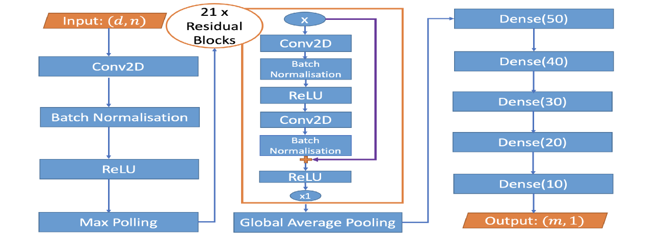
The image displays a flowchart-style block diagram illustrating the architecture of a deep convolutional neural network (CNN). The model processes an input of shape `(d, n)` through an initial convolutional block, followed by a stack of 21 residual blocks, and concludes with a series of fully connected (dense) layers to produce an output of shape `(m, 1)`. The diagram uses color-coded blocks (blue for processing layers, orange for input/output and the residual block container) and directional arrows to indicate data flow.
### Components/Axes
The diagram is organized into three primary vertical sections, flowing from left to right:
1. **Initial Processing Path (Left Column):**
* **Input:** An orange parallelogram labeled `Input: (d, n)`.
* **Layer 1:** A blue rectangle labeled `Conv2D`.
* **Layer 2:** A blue rectangle labeled `Batch Normalisation`.
* **Layer 3:** A blue rectangle labeled `ReLU`.
* **Layer 4:** A blue rectangle labeled `Max Polling` (Note: Likely a typo for "Pooling").
* An arrow connects the output of `Max Polling` to the next section.
2. **Residual Block Stack (Center Column):**
* **Container:** An orange-bordered rectangle encloses the structure of a single residual block. A label above it reads `21 x Residual Blocks`, indicating this block is repeated 21 times sequentially.
* **Internal Structure of One Residual Block:**
* **Input Node:** A blue oval labeled `x`.
* **Main Path:**
1. `Conv2D` (blue rectangle)
2. `Batch Normalisation` (blue rectangle)
3. `ReLU` (blue rectangle)
4. `Conv2D` (blue rectangle)
5. `Batch Normalisation` (blue rectangle)
* **Skip Connection:** A purple arrow originates from the input node `x`, bypasses the main path layers, and connects to an addition operation (represented by a small orange plus symbol `+`) after the second `Batch Normalisation`.
* **Final Activation:** A `ReLU` (blue rectangle) applied after the addition.
* **Output Node:** A blue oval labeled `x1`.
* The output of the 21st residual block (`x1`) flows to the next stage.
3. **Classification Head (Right Column):**
* **Pooling Layer:** A blue rectangle labeled `Global Average Pooling`. It receives the output from the residual stack.
* **Dense Layers:** A vertical stack of five blue rectangles, each representing a fully connected layer with a specified number of neurons:
1. `Dense(50)`
2. `Dense(40)`
3. `Dense(30)`
4. `Dense(20)`
5. `Dense(10)`
* **Output:** An orange parallelogram labeled `Output: (m, 1)`.
### Detailed Analysis
* **Data Flow:** The data flows unidirectionally from the `Input (d, n)` at the top-left, down through the initial block, then into the stack of 21 residual blocks, through global average pooling, down through the five dense layers, and finally to the `Output (m, 1)` at the bottom-right.
* **Layer Specifications:**
* **Convolutional Layers:** The diagram specifies `Conv2D` layers but does not provide kernel size, stride, or padding parameters.
* **Normalization:** `Batch Normalisation` is used consistently after convolutional layers.
* **Activation:** `ReLU` is the specified activation function, used both within the residual blocks and after the initial convolution.
* **Pooling:** Two types are used: `Max Polling` (likely 2D max pooling) early in the network and `Global Average Pooling` after the residual stack to reduce spatial dimensions before the dense layers.
* **Residual Block:** The block follows a standard pre-activation design (Conv->BN->ReLU->Conv->BN) with a skip connection that adds the original input `x` to the output of the second BN layer, followed by a final ReLU. The output is denoted `x1`.
* **Dense Layers:** The network progressively reduces the feature dimension through dense layers with neuron counts: 50 -> 40 -> 30 -> 20 -> 10.
* **Dimensions:**
* **Input:** `(d, n)` - This suggests a 2D input, possibly (height, width) for a single-channel image or (features, time) for a signal.
* **Output:** `(m, 1)` - This suggests a vector of `m` output values, typical for regression or multi-label classification tasks. The value of `m` is not specified.
### Key Observations
1. **Deep Residual Core:** The architecture's defining feature is the very deep stack of **21 identical residual blocks**. This is a significant depth, designed to learn highly complex, hierarchical features.
2. **Architectural Consistency:** The residual block design is uniform throughout the stack, with no variation in the number of filters or internal structure mentioned.
3. **Dimensionality Reduction:** The network employs a clear strategy for reducing spatial/feature dimensions: early max pooling, followed by global average pooling after the deep feature extractor, and finally a tapering sequence of dense layers.
4. **Potential Typo:** The label `Max Polling` is almost certainly a misspelling of `Max Pooling`.
5. **Lack of Specifics:** The diagram is a high-level architectural schematic. It omits critical implementation details such as the number of convolutional filters, kernel sizes, stride, padding, dropout rates, and the specific value of `m` for the output.
### Interpretation
This diagram represents a deep, purpose-built convolutional neural network designed for a task requiring the extraction of complex patterns from structured 2D input data (e.g., image analysis, spectrogram processing, or certain types of sensor data).
* **Purpose of Residual Blocks:** The use of 21 residual blocks with skip connections is a direct application of deep residual learning principles. This design mitigates the vanishing gradient problem, allowing the training of an extremely deep network. The network can learn identity mappings easily via the skip connections, enabling it to focus on learning residual functions that improve performance.
* **Feature Processing Pipeline:** The architecture follows a classic pattern: a shallow initial feature extraction (`Conv2D` -> `BN` -> `ReLU` -> `Max Pooling`), followed by a very deep feature refinement stage (the residual stack), and concluding with a task-specific regression/classification head (the dense layers). The `Global Average Pooling` layer is crucial for making the network invariant to spatial translations of features in the final feature map and for drastically reducing the number of parameters before the dense layers.
* **Output Implication:** The output shape `(m, 1)` suggests the model is designed for a task like multi-output regression (predicting `m` continuous values) or multi-label classification (predicting `m` independent binary labels). It is not structured for standard single-class classification (which would typically end with a softmax layer of size `C`).
* **Inferred Complexity:** The depth (21 residual blocks) implies this model is intended for a complex problem where a shallower network would underfit. However, the lack of specified filter counts makes it impossible to gauge the total parameter count and computational cost accurately. The tapering dense layers (50->10 neurons) suggest a deliberate compression of the high-level feature representation into a compact final vector for prediction.
DECODING INTELLIGENCE...