## [Composite Scientific Visualization]: Comparison of Turbulence Modeling Approaches for Flow Over a Backward-Facing Step
### Overview
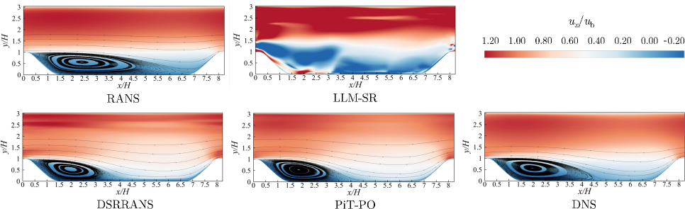
The image is a composite scientific visualization comparing five different computational methods for simulating turbulent flow over a backward-facing step. It consists of five individual contour plots (arranged in a 2x3 grid, with the sixth position occupied by a color bar legend) and a shared color scale. Each plot displays the normalized streamwise velocity field (`u_x/u_b`) overlaid with flow streamlines. The primary purpose is to visually compare the accuracy and characteristics of different turbulence models against a high-fidelity reference solution.
### Components/Axes
* **Layout:** Five data plots and one color bar legend. Top row (left to right): RANS, LLM-SR, Color Bar. Bottom row (left to right): DSRRANS, Pi-PO, DNS.
* **Axes (All Plots):**
* **X-axis:** Label: `x/H`. Scale: Linear, from 0 to 8. Ticks at intervals of 0.5.
* **Y-axis:** Label: `y/H`. Scale: Linear, from 0 to 3. Ticks at intervals of 0.5.
* **Color Bar Legend (Top Right):**
* **Variable:** `u_x/u_b` (Normalized streamwise velocity).
* **Scale:** Linear, ranging from -0.20 to 1.20.
* **Color Gradient:** Diverging scheme. Blue represents negative values (down to -0.20), transitioning through white at 0.00, to red for positive values (up to 1.20).
* **Tick Values:** -0.20, 0.00, 0.20, 0.40, 0.60, 0.80, 1.00, 1.20.
* **Plot Titles (Below each subplot):**
1. `RANS` (Top Left)
2. `LLM-SR` (Top Center)
3. `DSRRANS` (Bottom Left)
4. `Pi-PO` (Bottom Center)
5. `DNS` (Bottom Right)
### Detailed Analysis
Each subplot visualizes the same physical domain: flow moving from left to right over a step located at `x/H = 0`, `y/H = 1`. The streamlines show the path of fluid particles, and the color indicates local velocity.
1. **RANS (Top Left):**
* **Trend:** Shows a large, smooth, and stable recirculation zone (blue region) immediately behind the step. The reattachment point (where the flow reattaches to the bottom wall) appears to be around `x/H ≈ 6.5`.
* **Velocity Field:** The core flow above the step (red/orange) is relatively uniform. The recirculation zone is a deep, consistent blue, indicating strongly negative velocity.
2. **LLM-SR (Top Center):**
* **Trend:** Exhibits a highly irregular and chaotic flow field compared to all other methods. The recirculation zone is fragmented and not well-defined. There are patches of high and low velocity scattered throughout the domain.
* **Velocity Field:** Shows extreme variations, with intense red (high velocity) and blue (negative velocity) regions appearing in non-physical, patchy distributions. This suggests a potential instability or failure in this particular simulation/model.
3. **DSRRANS (Bottom Left):**
* **Trend:** Similar overall structure to RANS but with a slightly more detailed recirculation zone. The reattachment point is slightly further downstream, approximately `x/H ≈ 7.0`.
* **Velocity Field:** The recirculation zone is well-defined but shows more internal structure (lighter blue gradients) compared to the monolithic blue of RANS.
4. **Pi-PO (Bottom Center):**
* **Trend:** The recirculation zone is smaller and more compact than in RANS/DSRRANS. The reattachment point is significantly further upstream, around `x/H ≈ 5.5`.
* **Velocity Field:** The core flow above the step shows more pronounced velocity gradients (bands of orange and red). The recirculation zone is a distinct, concentrated blue oval.
5. **DNS (Bottom Right):**
* **Trend:** As the Direct Numerical Simulation (the high-fidelity reference), it shows the most complex and detailed flow structure. The recirculation zone has a complex internal vortex structure. The reattachment point is approximately `x/H ≈ 6.0`.
* **Velocity Field:** Displays the finest gradients and most intricate streamline patterns, capturing small-scale turbulent structures not fully resolved by the other models.
### Key Observations
* **Model Discrepancy:** There is significant variation in the predicted size, shape, and internal structure of the recirculation zone across the five methods.
* **LLM-SR Anomaly:** The LLM-SR result is a clear outlier, showing a physically implausible, noisy flow field that does not resemble the coherent structures seen in the other models or the DNS reference.
* **Reattachment Point Variation:** The estimated reattachment point varies considerably: Pi-PO (~5.5) < DNS (~6.0) < RANS (~6.5) < DSRRANS (~7.0).
* **Structural Fidelity:** DNS shows the most detailed vortex core within the recirculation zone. DSRRANS and Pi-PO capture some internal structure, while RANS shows a more simplified, monolithic vortex.
### Interpretation
This visualization is a comparative study of turbulence modeling fidelity. The **DNS** plot serves as the ground truth. The **RANS** model, a traditional workhorse, provides a stable but overly smoothed and slightly inaccurate prediction (overestimating reattachment length). **DSRRANS** appears to be a variant that adds some detail but still overpredicts the recirculation zone size. **Pi-PO** underpredicts the zone size, suggesting a different bias in its modeling approach.
The most striking result is the **LLM-SR** model. Its output is not just inaccurate but qualitatively different, exhibiting a lack of physical coherence. This suggests that this particular application of a Large Language Model (or similar ML approach) to this fluid dynamics problem may be unstable, improperly trained, or fundamentally unsuited for capturing the continuous, physics-governed nature of this flow field. The image effectively demonstrates that while advanced models (like DSRRANS, Pi-PO) can modulate the predictions of traditional RANS, not all novel approaches (like this LLM-SR instance) yield physically plausible results. The core takeaway is the critical importance of validation against high-fidelity data (DNS) when developing or applying new computational models.