## Scatter Plot Grid: Scaling Relationships
### Overview
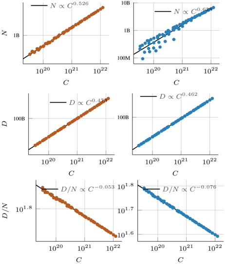
The image displays a 3x2 grid of six scatter plots, each illustrating a power-law relationship between variables on logarithmic axes. The plots are organized into two columns (left: orange data points, right: blue data points) and three rows (top: N vs. C, middle: D vs. C, bottom: D/N vs. C). Each plot includes a fitted trend line with its corresponding proportionality equation.
### Components/Axes
* **Grid Structure:** 3 rows × 2 columns.
* **Common X-Axis (All Plots):** Labeled **C**. Scale is logarithmic, with major tick marks at `10^20`, `10^21`, and `10^22`.
* **Y-Axes (Row-Specific):**
* **Top Row:** Labeled **N**. Scale is logarithmic. Left plot ticks: `1B` (10^9), `10B` (10^10). Right plot ticks: `100M` (10^8), `1B` (10^9), `10B` (10^10).
* **Middle Row:** Labeled **D**. Scale is logarithmic. Left plot tick: `100B` (10^11). Right plot tick: `100B` (10^11).
* **Bottom Row:** Labeled **D/N**. Scale is logarithmic. Left plot ticks: `10^1.6`, `10^1.7`, `10^1.8`. Right plot ticks: `10^1.6`, `10^1.7`, `10^1.8`.
* **Legends (Within each plot):** A black line segment with text indicating the fitted power-law relationship.
* **Data Series:**
* **Left Column (Orange):** Data points are orange circles.
* **Right Column (Blue):** Data points are blue circles.
### Detailed Analysis
**Row 1: N vs. C**
* **Top-Left Plot (Orange):**
* **Trend:** A strong, positive linear trend on the log-log plot, indicating a power-law relationship. The line slopes upward from left to right.
* **Equation:** `N ∝ C^0.526`
* **Data Range:** C spans from approximately `5×10^19` to `2×10^22`. N spans from just below `1B` to just above `10B`.
* **Top-Right Plot (Blue):**
* **Trend:** A positive linear trend, but with more scatter than the orange dataset. The line slopes upward.
* **Equation:** `N ∝ C^0.684`
* **Data Range:** C spans from approximately `5×10^19` to `2×10^22`. N spans from below `100M` to near `10B`.
**Row 2: D vs. C**
* **Middle-Left Plot (Orange):**
* **Trend:** A strong, positive linear trend. The line slopes upward.
* **Equation:** `D ∝ C^0.472`
* **Data Range:** C spans from approximately `5×10^19` to `2×10^22`. D is centered around `100B`.
* **Middle-Right Plot (Blue):**
* **Trend:** A strong, positive linear trend. The line slopes upward.
* **Equation:** `D ∝ C^0.462`
* **Data Range:** C spans from approximately `5×10^19` to `2×10^22`. D is centered around `100B`.
**Row 3: D/N vs. C**
* **Bottom-Left Plot (Orange):**
* **Trend:** A strong, negative linear trend on the log-log plot. The line slopes downward from left to right.
* **Equation:** `D/N ∝ C^(-0.053)`
* **Data Range:** C spans from approximately `5×10^19` to `2×10^22`. D/N decreases from near `10^1.8` to near `10^1.6`.
* **Bottom-Right Plot (Blue):**
* **Trend:** A strong, negative linear trend. The line slopes downward.
* **Equation:** `D/N ∝ C^(-0.076)`
* **Data Range:** C spans from approximately `5×10^19` to `2×10^22`. D/N decreases from near `10^1.8` to near `10^1.6`.
### Key Observations
1. **Consistent Scaling:** All six plots demonstrate clear power-law scaling (linear on log-log axes).
2. **Variable Growth:** Both `N` and `D` increase with `C`, but `N` grows faster than `D` in both datasets (exponents for N: 0.526, 0.684 > exponents for D: 0.472, 0.462).
3. **Declining Ratio:** Consequently, the ratio `D/N` decreases as `C` increases for both datasets (negative exponents: -0.053, -0.076).
4. **Dataset Comparison:** The blue dataset (right column) shows a stronger scaling of `N` with `C` (exponent 0.684 vs. 0.526) but a slightly weaker scaling of `D` with `C` (0.462 vs. 0.472) compared to the orange dataset. This leads to a more pronounced decline in `D/N` for the blue dataset (exponent -0.076 vs. -0.053).
5. **Data Scatter:** The `N vs. C` plot for the blue dataset exhibits significantly more variance around the trend line compared to the other five plots.
### Interpretation
The data suggests fundamental scaling laws governing the relationship between a quantity `C` (likely a measure of compute, cost, or capacity) and two other metrics, `N` (perhaps number of parameters or components) and `D` (perhaps dataset size or another resource).
* **Sub-linear Scaling:** The exponents for `N` and `D` are all less than 1, indicating sub-linear growth. Doubling `C` does not double `N` or `D`; it increases them by a smaller factor (e.g., `2^0.526 ≈ 1.44` for `N` in the orange dataset).
* **Efficiency Trend:** The decreasing `D/N` ratio implies that as systems scale up with `C`, the resource `D` per unit of `N` diminishes. This could reflect increasing efficiency, a shift in resource allocation, or a saturation effect.
* **Dataset Divergence:** The two columns (orange vs. blue) likely represent two different model families, training regimes, or technological generations. The blue dataset's steeper `N(C)` scaling suggests a paradigm that more aggressively increases `N` with `C`, while its slightly flatter `D(C)` scaling and steeper decline in `D/N` suggest a different strategy for balancing `N` and `D` during scaling.
* **Predictive Power:** These fitted power laws (`N ∝ C^α`, `D ∝ C^β`, `D/N ∝ C^(β-α)`) provide a quantitative framework for predicting how system characteristics (`N`, `D`) will evolve with increased `C`, which is crucial for planning and research in fields like machine learning, engineering, or economics where such scaling is studied.