## Diagram: Scale Factor and Binary Weight Matrix Configuration
### Overview
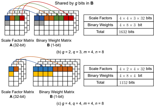
The image presents two technical diagrams (labeled **b** and **c**) illustrating the configuration of **Scale Factor Matrix A** (32-bit) and **Binary Weight Matrix B** (1-bit), with shared bits in B. Each diagram includes a table summarizing the bit allocation for scale factors, binary weights, and total bits. The diagrams use color-coded arrows to indicate shared bits and spatial relationships between matrices.
---
### Components/Axes
1. **Matrices**:
- **Scale Factor Matrix A**: 32-bit values, represented as a grid with colored blocks (blue, orange, green, red).
- **Binary Weight Matrix B**: 1-bit values, represented as a grid with uniform blocks.
- Arrows connect Scale Factor Matrix A to Binary Weight Matrix B, labeled "Shared by *g* bits in B."
2. **Tables**:
- **Scale Factors**: Dimensions and total bits (e.g., `4 × 4 × 3 × 32 bits`).
- **Binary Weights**: Dimensions and total bits (e.g., `4 × 8 × 3 bits`).
- **Total**: Sum of scale factors and binary weights (e.g., `1632 bits`).
3. **Parameters**:
- **g**: Number of shared bits in B (e.g., `g = 2` in diagram **b**, `g = 4` in diagram **c**).
- **q, m, n**: Dimensions influencing matrix sizes (e.g., `q = 3`, `m = 4`, `n = 8` in diagram **b**).
---
### Detailed Analysis
#### Diagram **b** (`g = 2`, `q = 3`, `m = 4`, `n = 8`):
- **Scale Factors**: `4 × 4 × 3 × 32 bits`
- Total: `4 × 4 × 3 × 32 = 1,536 bits`.
- **Binary Weights**: `4 × 8 × 3 bits`
- Total: `4 × 8 × 3 = 96 bits`.
- **Total**: `1,536 + 96 = 1,632 bits`.
#### Diagram **c** (`g = 4`, `q = 4`, `m = 4`, `n = 8`):
- **Scale Factors**: `4 × 2 × 4 × 32 bits`
- Total: `4 × 2 × 4 × 32 = 1,024 bits`.
- **Binary Weights**: `4 × 8 × 4 bits`
- Total: `4 × 8 × 4 = 128 bits`.
- **Total**: `1,024 + 128 = 1,152 bits`.
**Key Observations**:
1. **Shared Bits (`g`)**:
- In **b**, `g = 2` bits are shared between A and B.
- In **c**, `g = 4` bits are shared, reducing redundancy.
2. **Matrix Dimensions**:
- Scale Factor Matrix A’s first dimension scales as `n/g` (e.g., `8/2 = 4` in **b**, `8/4 = 2` in **c**).
- Binary Weight Matrix B’s third dimension scales with `q` (e.g., `q = 3` in **b**, `q = 4` in **c**).
3. **Total Bit Reduction**: Increasing `g` from 2 to 4 reduces total bits from 1,632 to 1,152, demonstrating efficiency gains from shared bits.
---
### Interpretation
1. **Efficiency Trade-offs**:
- Higher `g` values (shared bits) reduce the Scale Factor Matrix size (`n/g`) but increase Binary Weight Matrix size (`q`). However, the net effect is lower total bits, suggesting optimized memory usage.
- Example: In **c**, doubling `g` (from 2 to 4) halves the Scale Factor dimension (`4 → 2`) while increasing Binary Weights (`3 → 4`), but total bits drop by 30%.
2. **Hardware Implications**:
- This configuration likely targets applications like neural networks, where 32-bit precision (Scale Factors) and 1-bit weights (Binary Weights) balance accuracy and efficiency.
- Shared bits (`g`) may represent quantized or compressed data paths, critical for low-power hardware.
3. **Anomalies**:
- No outliers; trends align with parameter definitions. The reduction in total bits with higher `g` is consistent across diagrams.
---
### Key Takeaways
- **Shared Bits (`g`)**: Directly impact memory efficiency by reducing Scale Factor dimensions while increasing Binary Weight granularity.
- **Parameter Interplay**: `n`, `q`, and `m` define matrix sizes, with `g` acting as a compression factor.
- **Practical Use**: Enables efficient storage and computation in hardware-accelerated AI models, balancing precision and resource constraints.