# Technical Document Extraction: KAN Model Performance Analysis
## Main Title
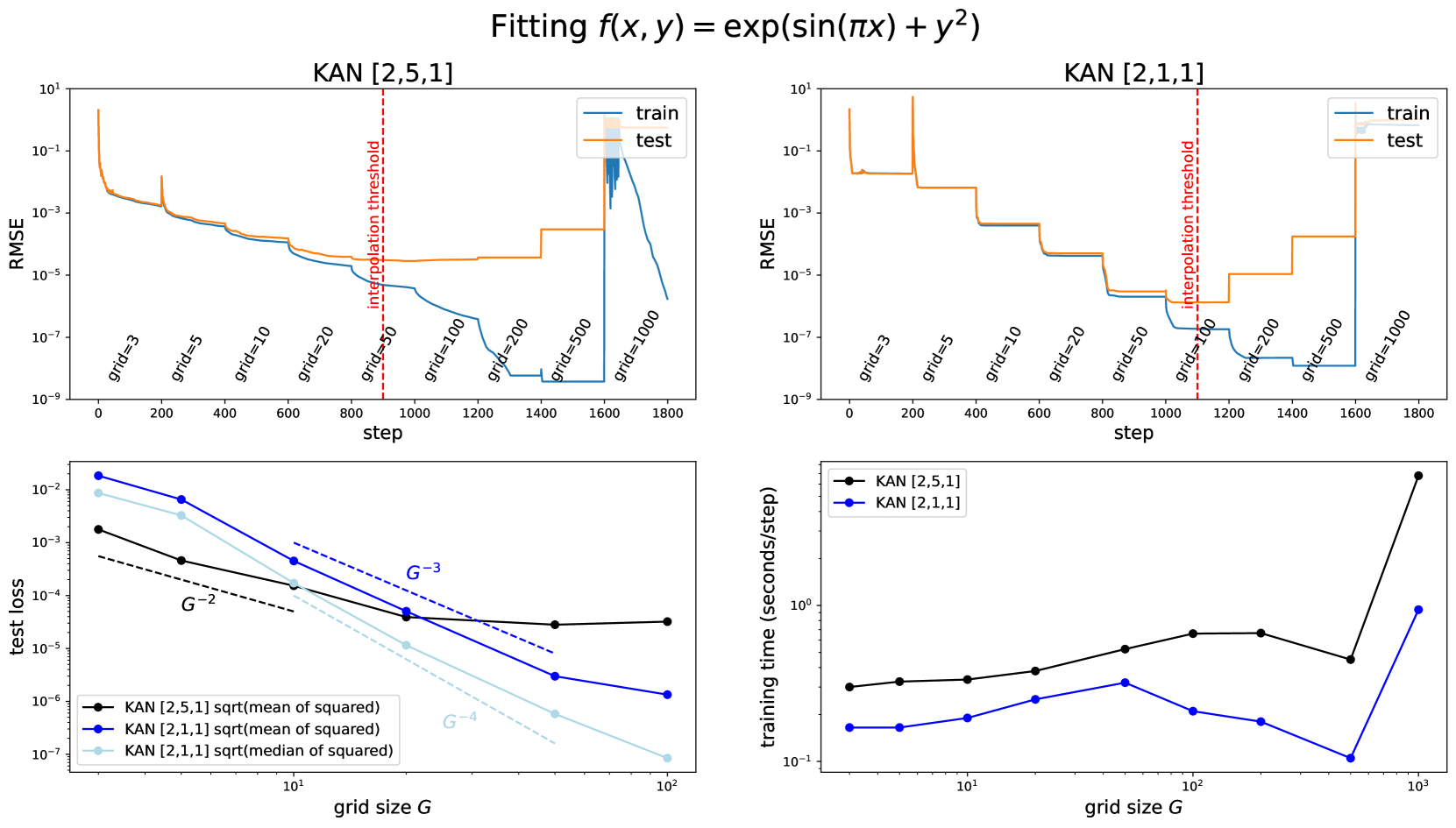
Fitting f(x, y) = exp(sin(πx)) + y²
---
### Top Left Graph: KAN [2,5,1]
#### Axes
- **X-axis**: `step` (0 to 1800)
- **Y-axis**: `RMSE` (log scale: 10⁻⁹ to 10¹)
#### Legend
- `train` (blue line)
- `test` (orange line)
#### Key Elements
- Red dashed vertical line labeled `interpolation threshold`
- Grid size annotations: `grid=3`, `grid=5`, `grid=10`, `grid=20`, `grid=50`, `grid=100`, `grid=200`, `grid=500`, `grid=1000`
#### Trends
- **Train RMSE**: Gradual decline with minor fluctuations.
- **Test RMSE**: Sharp spikes at `grid=500` and `grid=1000`, followed by steep drops.
- Interpolation threshold occurs near `step=1000`.
---
### Top Right Graph: KAN [2,1,1]
#### Axes
- **X-axis**: `step` (0 to 1800)
- **Y-axis**: `RMSE` (log scale: 10⁻⁹ to 10¹)
#### Legend
- `train` (blue line)
- `test` (orange line)
#### Key Elements
- Red dashed vertical line labeled `interpolation threshold`
- Grid size annotations: `grid=3`, `grid=5`, `grid=10`, `grid=20`, `grid=50`, `grid=100`, `grid=200`, `grid=500`, `grid=1000`
#### Trends
- **Train RMSE**: Stable until `step=1000`, then sharp decline.
- **Test RMSE**: Multiple plateaus and spikes, with a critical rise at `grid=1000`.
---
### Bottom Left Graph: Training Loss vs Grid Size G
#### Axes
- **X-axis**: `grid size G` (log scale: 10¹ to 10²)
- **Y-axis**: `test loss` (log scale: 10⁻⁶ to 10⁻²)
#### Legend
- `KAN [2,5,1] sqrt(mean of squared)` (black line)
- `KAN [2,1,1] sqrt(mean of squared)` (blue line)
- `KAN [2,1,1] sqrt(median of squared)` (light blue line)
#### Annotations
- Dashed lines labeled `G⁻²`, `G⁻³`, `G⁻⁴`
#### Trends
- All models show decaying loss with increasing G.
- `KAN [2,1,1] sqrt(median of squared)` decays fastest (aligns with `G⁻⁴`).
---
### Bottom Right Graph: Training Time vs Grid Size G
#### Axes
- **X-axis**: `grid size G` (log scale: 10¹ to 10³)
- **Y-axis**: `training time (seconds/step)` (log scale: 10⁻¹ to 10¹)
#### Legend
- `KAN [2,5,1]` (black line)
- `KAN [2,1,1]` (blue line)
#### Trends
- **KAN [2,5,1]**: Gradual increase, sharp spike at `G=1000`.
- **KAN [2,1,1]**: Slower growth, with a plateau at `G=100`.
---
### Cross-Referenced Observations
1. **Interpolation Threshold**:
- Both top graphs show a red dashed line at `step=1000`, indicating a critical point for model performance.
2. **Grid Size Impact**:
- Larger grid sizes (e.g., `G=1000`) correlate with higher test RMSE spikes and longer training times.
3. **Model Complexity**:
- `KAN [2,5,1]` exhibits higher training times and more volatile test RMSE compared to `KAN [2,1,1]`.
4. **Loss Metrics**:
- `sqrt(median of squared)` loss metric for `KAN [2,1,1]` achieves the fastest decay (G⁻⁴).
---
### Summary
The graphs illustrate the trade-offs between model complexity (grid size) and performance metrics (RMSE, training loss, training time). `KAN [2,1,1]` with `sqrt(median of squared)` loss demonstrates optimal efficiency, while `KAN [2,5,1]` requires careful grid size selection to avoid overfitting and excessive computational cost.