TECHNICAL ASSET FINGERPRINT
99cd19c61544fdb0df9c1ed4
Click to view fullscreen
Press ESC or click to close
FOUND IN PAPERS
EXPERT: healer-alpha-free VERSION 1
RUNTIME: free/openrouter/healer-alpha
INTEL_VERIFIED
## Multi-Panel Line Chart: Model Size vs. Accuracy Across Decomposition Methods
### Overview
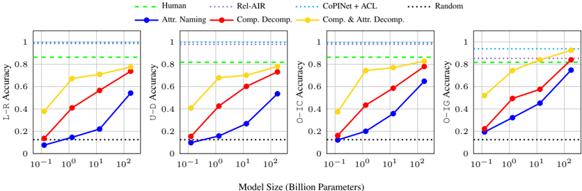
The image displays a set of four horizontally arranged line charts, each plotting "Accuracy" (y-axis) against "Model Size (Billion Parameters)" (x-axis, logarithmic scale). The charts compare the performance of different computational models and human baselines on four distinct tasks or metrics: L-R Accuracy, U-D Accuracy, O-IC Accuracy, and O-IG Accuracy. The primary variable is model size, and the lines represent different methods or baselines.
### Components/Axes
* **Common X-Axis (Bottom Center):** "Model Size (Billion Parameters)". Scale is logarithmic, with major tick marks at `10^-1` (0.1), `10^0` (1), `10^1` (10), and `10^2` (100).
* **Individual Y-Axes (Left of each subplot):**
* Leftmost Chart: "L-R Accuracy"
* Second Chart: "U-D Accuracy"
* Third Chart: "O-IC Accuracy"
* Rightmost Chart: "O-IG Accuracy"
* All y-axes share the same scale from 0 to 1, with major ticks at 0, 0.2, 0.4, 0.6, 0.8, and 1.0.
* **Legend (Top Center, spanning all charts):**
* **Human:** Green dashed line (`--`).
* **Rel-AIR:** Purple dotted line (`...`).
* **CoPINet + ACL:** Cyan/Light blue dotted line (`...`).
* **Random:** Black dotted line (`...`).
* **Attr. Naming:** Blue solid line with circle markers (`-o`).
* **Comp. Decomp.:** Red solid line with circle markers (`-o`).
* **Comp. & Attr. Decomp.:** Yellow/Gold solid line with circle markers (`-o`).
### Detailed Analysis
Data points are estimated from the visual plots. Values are approximate.
**1. L-R Accuracy Chart (Leftmost):**
* **Trend:** All three solid-line methods show a clear, monotonic increase in accuracy with model size.
* **Data Points (Approximate):**
* **Comp. & Attr. Decomp. (Yellow):** 0.1B: ~0.40 | 1B: ~0.68 | 10B: ~0.72 | 100B: ~0.88
* **Comp. Decomp. (Red):** 0.1B: ~0.15 | 1B: ~0.42 | 10B: ~0.58 | 100B: ~0.75
* **Attr. Naming (Blue):** 0.1B: ~0.08 | 1B: ~0.15 | 10B: ~0.22 | 100B: ~0.55
* **Baselines (Horizontal Lines):**
* **Human (Green):** Constant at ~0.85.
* **Rel-AIR (Purple):** Constant at ~0.98.
* **CoPINet + ACL (Cyan):** Constant at ~1.00.
* **Random (Black):** Constant at ~0.12.
**2. U-D Accuracy Chart (Second from Left):**
* **Trend:** Similar increasing trend for solid lines. The yellow line shows a sharp initial increase.
* **Data Points (Approximate):**
* **Comp. & Attr. Decomp. (Yellow):** 0.1B: ~0.42 | 1B: ~0.68 | 10B: ~0.72 | 100B: ~0.82
* **Comp. Decomp. (Red):** 0.1B: ~0.15 | 1B: ~0.42 | 10B: ~0.62 | 100B: ~0.75
* **Attr. Naming (Blue):** 0.1B: ~0.08 | 1B: ~0.15 | 10B: ~0.28 | 100B: ~0.55
* **Baselines:** Identical constant values as in the L-R chart.
**3. O-IC Accuracy Chart (Third from Left):**
* **Trend:** Strong, consistent upward trends. The yellow line approaches the human baseline at 100B parameters.
* **Data Points (Approximate):**
* **Comp. & Attr. Decomp. (Yellow):** 0.1B: ~0.40 | 1B: ~0.75 | 10B: ~0.78 | 100B: ~0.85
* **Comp. Decomp. (Red):** 0.1B: ~0.15 | 1B: ~0.48 | 10B: ~0.62 | 100B: ~0.80
* **Attr. Naming (Blue):** 0.1B: ~0.12 | 1B: ~0.20 | 10B: ~0.38 | 100B: ~0.65
* **Baselines:** Identical constant values as in the L-R chart.
**4. O-IG Accuracy Chart (Rightmost):**
* **Trend:** The most pronounced upward trends. The yellow line surpasses the human baseline between 10B and 100B parameters.
* **Data Points (Approximate):**
* **Comp. & Attr. Decomp. (Yellow):** 0.1B: ~0.52 | 1B: ~0.70 | 10B: ~0.82 | 100B: ~0.92
* **Comp. Decomp. (Red):** 0.1B: ~0.22 | 1B: ~0.50 | 10B: ~0.58 | 100B: ~0.85
* **Attr. Naming (Blue):** 0.1B: ~0.20 | 1B: ~0.35 | 10B: ~0.45 | 100B: ~0.75
* **Baselines:** Identical constant values as in the L-R chart.
### Key Observations
1. **Performance Hierarchy:** Across all four tasks and nearly all model sizes, the method hierarchy is consistent: `Comp. & Attr. Decomp.` (Yellow) > `Comp. Decomp.` (Red) > `Attr. Naming` (Blue).
2. **Scaling Law:** All three model-based methods (solid lines) exhibit a clear positive correlation between model size (log scale) and accuracy. The relationship appears roughly linear on this semi-log plot, suggesting a power-law relationship between parameters and performance.
3. **Baseline Comparison:** The `Random` baseline is consistently low (~0.12). The `Human` baseline (~0.85) is a significant target that the best model (`Comp. & Attr. Decomp.`) approaches or exceeds at the largest scale (100B), particularly in the O-IG task.
4. **Task Difficulty:** The starting performance (at 0.1B) and the slope of improvement vary by task. The O-IG task shows the highest starting point and steepest climb for the best method, while L-R and U-D show more gradual improvement.
5. **Saturation of Baselines:** The `Rel-AIR` and `CoPINet + ACL` methods perform at or near ceiling (~0.98-1.00) regardless of the model size axis, indicating they are either not dependent on this scaling factor or represent a different class of solution.
### Interpretation
This set of charts provides a Peircean investigation into the relationship between **model scale**, **architectural approach** (decomposition strategy), and **task performance** in what appears to be a visual or relational reasoning benchmark.
* **The Sign (Data):** The consistent upward trends are an index of learning and capacity increase with scale. The strict ordering of the colored lines is a symbol of the relative efficacy of the decomposition strategies.
* **The Icon (Resemblance):** The charts visually model the "learning curve" of AI systems. The gap between the blue line (`Attr. Naming`) and the yellow line (`Comp. & Attr. Decomp.`) iconically represents the performance gain achieved by incorporating compositional decomposition into the model's reasoning process.
* **The Interpretant (Meaning):** The data suggests that **compositional decomposition is a critical inductive bias** for these tasks. Merely naming attributes (`Attr. Naming`) is insufficient. The most effective approach (`Comp. & Attr. Decomp.`) combines both understanding of parts (composition) and their properties (attributes). Furthermore, the benefits of this architectural bias **scale with model size**, allowing large models to match or surpass human-level performance on specific subtasks (O-IG). The flat, high-performing baselines (`Rel-AIR`, `CoPINet+ACL`) likely represent specialized, non-scaling algorithms, highlighting a trade-off between general scalable learning and specialized engineered solutions. The charts argue that for generalizable reasoning, scale combined with the right structural priors (decomposition) is a powerful path forward.
DECODING INTELLIGENCE...