## Line Chart: Accuracy vs. Time with Varying Parameters ### Overview The image is a line chart that plots the test accuracy (Acc_test) against time (t) for different values of parameters lambda (λ^s) and r. The chart shows how the accuracy changes over time for different configurations of these parameters. ### Components/Axes * **X-axis:** Time (t), ranging from -1 to 4. * **Y-axis:** Test Accuracy (Acc_test), ranging from 0.4 to 1.0. * **Legend (Top-Left):** * Cyan: λ^s = 2 * Blue: λ^s = 1 * Dark Blue: λ^s = 0.5 * Yellow: r = 10^3 * Olive: r = 10^2 * Brown: r = 10^1 * Purple: r = 10^0 ### Detailed Analysis * **λ^s = 2 (Cyan):** The line starts at approximately 0.4 at t = -1, increases sharply to approximately 0.98 at t = 1, and then remains relatively constant around 0.98 until t = 4. * **λ^s = 1 (Blue):** The line starts at approximately 0.42 at t = -1, increases sharply to approximately 0.8 at t = 1, and then decreases slightly to approximately 0.74 at t = 4. * **λ^s = 0.5 (Dark Blue):** The line starts at approximately 0.4 at t = -1, increases to approximately 0.67 at t = 1, and then decreases to approximately 0.6 at t = 4. * **r = 10^3 (Yellow):** The data points start at approximately 0.4 at t = -1, increase to approximately 0.7 at t = 1, and then fluctuate between 0.7 and 0.8 until t = 4. * **r = 10^2 (Olive):** The data points start at approximately 0.4 at t = -1, increase to approximately 0.75 at t = 1, and then fluctuate between 0.75 and 0.85 until t = 4. * **r = 10^1 (Brown):** The data points start at approximately 0.4 at t = -1, increase to approximately 0.8 at t = 1, and then fluctuate between 0.8 and 0.9 until t = 4. * **r = 10^0 (Purple):** The data points start at approximately 0.4 at t = -1, increase to approximately 0.85 at t = 1, and then fluctuate between 0.85 and 0.95 until t = 4. ### Key Observations * The lines representing different values of λ^s show a smooth transition, while the data points representing different values of r show more fluctuation. * Higher values of λ^s generally lead to higher test accuracy. * Higher values of r generally lead to higher test accuracy. * The test accuracy increases sharply between t = -1 and t = 1 for all values of λ^s and r. * The test accuracy tends to stabilize or slightly decrease after t = 1. ### Interpretation The chart demonstrates the impact of parameters λ^s and r on the test accuracy of a model over time. The parameter λ^s appears to have a more consistent and predictable effect on the accuracy, as indicated by the smooth lines. The parameter r, on the other hand, shows more fluctuation in the accuracy, suggesting a less stable or more sensitive relationship. The initial increase in accuracy for all parameter values indicates a learning phase, while the subsequent stabilization or decrease suggests potential overfitting or diminishing returns. The higher accuracy achieved with larger λ^s and r values suggests that these parameters may be important for optimizing the model's performance. ```

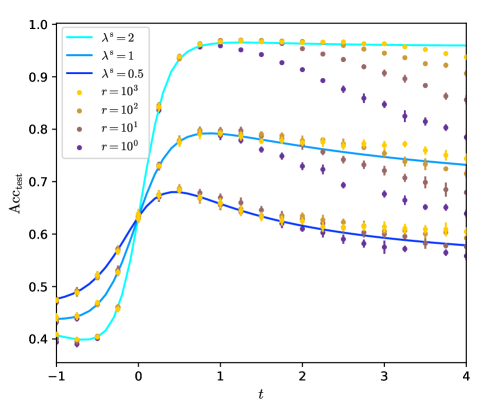
\n ## Line Chart: Acc_test vs. t for Different Lambda and r Values ### Overview This image presents a line chart illustrating the relationship between `Acc_test` (test accuracy) and `t` (time) for various values of lambda (λ⁰) and r. The chart displays multiple lines representing different parameter settings, allowing for a comparison of their performance over time. ### Components/Axes * **X-axis:** `t` (Time), ranging from approximately -1 to 4. * **Y-axis:** `Acc_test` (Test Accuracy), ranging from approximately 0.4 to 1.0. * **Legend:** Located in the top-left corner, identifying each line with its corresponding parameter values. * λ⁰ = 2 (Light Blue) * λ⁰ = 1 (Blue) * λ⁰ = 0.5 (Dark Blue) * r = 10³ (Yellow) * r = 10² (Orange) * r = 10⁰ (Purple) ### Detailed Analysis Here's a breakdown of each line's trend and approximate data points, cross-referencing with the legend colors: * **λ⁰ = 2 (Light Blue):** This line exhibits a steep upward slope initially, rapidly increasing from approximately 0.4 at t = -1 to nearly 1.0 by t = 1. It then plateaus, remaining relatively stable around 0.98-1.0 for the rest of the observed time. * t = -1, Acc_test ≈ 0.4 * t = 0, Acc_test ≈ 0.65 * t = 1, Acc_test ≈ 0.98 * t = 2, Acc_test ≈ 0.99 * t = 3, Acc_test ≈ 0.99 * t = 4, Acc_test ≈ 0.99 * **λ⁰ = 1 (Blue):** This line also shows an upward trend, but it's less steep than the λ⁰ = 2 line. It starts around 0.45 at t = -1 and reaches approximately 0.9 by t = 1. It then levels off, fluctuating around 0.9. * t = -1, Acc_test ≈ 0.45 * t = 0, Acc_test ≈ 0.6 * t = 1, Acc_test ≈ 0.9 * t = 2, Acc_test ≈ 0.91 * t = 3, Acc_test ≈ 0.9 * t = 4, Acc_test ≈ 0.9 * **λ⁰ = 0.5 (Dark Blue):** This line has the slowest initial increase. It begins around 0.48 at t = -1 and reaches approximately 0.7 by t = 1. It then plateaus around 0.7. * t = -1, Acc_test ≈ 0.48 * t = 0, Acc_test ≈ 0.55 * t = 1, Acc_test ≈ 0.7 * t = 2, Acc_test ≈ 0.7 * t = 3, Acc_test ≈ 0.7 * t = 4, Acc_test ≈ 0.7 * **r = 10³ (Yellow):** This line initially increases from approximately 0.45 at t = -1 to around 0.8 by t = 1. It then fluctuates around 0.8, showing some variability. * t = -1, Acc_test ≈ 0.45 * t = 0, Acc_test ≈ 0.6 * t = 1, Acc_test ≈ 0.8 * t = 2, Acc_test ≈ 0.78 * t = 3, Acc_test ≈ 0.78 * t = 4, Acc_test ≈ 0.78 * **r = 10² (Orange):** This line starts around 0.5 at t = -1 and increases to approximately 0.78 by t = 1. It then fluctuates around 0.75-0.8. * t = -1, Acc_test ≈ 0.5 * t = 0, Acc_test ≈ 0.6 * t = 1, Acc_test ≈ 0.78 * t = 2, Acc_test ≈ 0.76 * t = 3, Acc_test ≈ 0.76 * t = 4, Acc_test ≈ 0.76 * **r = 10⁰ (Purple):** This line exhibits a more erratic pattern. It starts around 0.48 at t = -1, increases to approximately 0.7 by t = 1, and then fluctuates significantly, decreasing to around 0.6 at t = 3 and then increasing again. * t = -1, Acc_test ≈ 0.48 * t = 0, Acc_test ≈ 0.6 * t = 1, Acc_test ≈ 0.7 * t = 2, Acc_test ≈ 0.75 * t = 3, Acc_test ≈ 0.6 * t = 4, Acc_test ≈ 0.7 ### Key Observations * Higher values of λ⁰ (2 and 1) lead to faster convergence to high accuracy. * The line for r = 10³ shows a relatively stable accuracy after the initial increase. * The line for r = 10⁰ exhibits the most variability in accuracy over time. * The lines for r = 10² and r = 10³ are relatively close to each other. ### Interpretation The chart demonstrates the impact of different parameter settings (λ⁰ and r) on the test accuracy (`Acc_test`) of a model over time (`t`). The results suggest that a larger λ⁰ value leads to faster learning and higher accuracy. The parameter 'r' appears to have a less pronounced effect, with values of 10³ and 10² resulting in similar performance. The erratic behavior of the r = 10⁰ line suggests that this parameter setting may be unstable or sensitive to initial conditions. The rapid increase in accuracy for higher λ⁰ values could indicate a faster learning rate, while the fluctuations in the r = 10⁰ line might be due to overfitting or underfitting. The plateauing of the lines after a certain time suggests that the models have converged to a stable state. This data could be used to optimize the parameter settings for the model to achieve the best possible performance.

## Line Chart: Test Accuracy vs. Parameter `t` for Different Model Configurations ### Overview The image is a line chart with error bars, plotting test accuracy (`Acc_test`) against a parameter `t`. It compares the performance of models configured with different values of a regularization or scaling parameter `λ^s` (lambda superscript s) and a parameter `r`. The chart demonstrates how accuracy evolves as `t` increases from -1 to 4 for each configuration. ### Components/Axes * **X-Axis:** Labeled `t`. Linear scale ranging from -1 to 4, with major tick marks at -1, 0, 1, 2, 3, 4. * **Y-Axis:** Labeled `Acc_test`. Linear scale ranging from 0.4 to 1.0, with major tick marks at 0.4, 0.5, 0.6, 0.7, 0.8, 0.9, 1.0. * **Legend (Top-Left Corner):** Contains two distinct groups: 1. **Lines (Solid):** Represent different values of `λ^s`. * Cyan line: `λ^s = 2` * Light blue line: `λ^s = 1` * Dark blue line: `λ^s = 0.5` 2. **Markers (Circles with Error Bars):** Represent different values of `r`. * Yellow circle: `r = 10^3` * Gold circle: `r = 10^2` * Brown circle: `r = 10^1` * Purple circle: `r = 10^0` ### Detailed Analysis **Data Series Trends (Lines):** 1. **`λ^s = 2` (Cyan Line):** Shows a steep, sigmoidal increase from `t = -1` (Acc ≈ 0.40) to `t ≈ 0.5`, then plateaus near the maximum accuracy of ~0.97 for `t > 1`. It maintains the highest accuracy across most of the `t` range. 2. **`λ^s = 1` (Light Blue Line):** Increases from `t = -1` (Acc ≈ 0.44) to a peak of ~0.80 at `t ≈ 0.5`, then gradually declines to ~0.73 at `t = 4`. 3. **`λ^s = 0.5` (Dark Blue Line):** Increases from `t = -1` (Acc ≈ 0.48) to a peak of ~0.68 at `t ≈ 0.2`, then declines more steeply to ~0.58 at `t = 4`. **Data Points by `r` Value (Markers):** * **General Pattern:** For a given `t` and `λ^s` line, higher `r` values (e.g., `10^3`, yellow) consistently yield higher accuracy points than lower `r` values (e.g., `10^0`, purple). The vertical spread of markers at a given `t` illustrates the impact of `r`. * **`r = 10^3` (Yellow):** Points cluster very closely to the `λ^s = 2` line, especially for `t > 0`. At `t=4`, accuracy is ~0.97. * **`r = 10^2` (Gold):** Points generally lie slightly below the `λ^s = 2` line and above the `λ^s = 1` line. At `t=4`, accuracy is ~0.95. * **`r = 10^1` (Brown):** Points show significant scatter. They are near the `λ^s = 1` line for `t < 1` but fall below it for larger `t`. At `t=4`, accuracy is ~0.82. * **`r = 10^0` (Purple):** Points exhibit the highest variance and lowest accuracy. They are consistently the lowest set of points. At `t=4`, accuracy is ~0.65. * **Error Bars:** Vertical error bars are present on all markers, indicating variability in the accuracy measurement. The bars appear larger for lower `r` values (e.g., `r=10^0`, purple) and for points where the trend is changing rapidly (e.g., near `t=0`). ### Key Observations 1. **Dominant Trend:** The `λ^s = 2` configuration achieves the highest and most stable test accuracy for `t > 0.5`. 2. **Parameter Interaction:** The benefit of a higher `r` value is most pronounced for the `λ^s = 2` configuration. For `λ^s = 0.5` and `λ^s = 1`, the performance gap between different `r` values narrows as `t` increases. 3. **Peak and Decline:** Both the `λ^s = 1` and `λ^s = 0.5` series show a clear peak in accuracy at low `t` values (`t ≈ 0.5` and `t ≈ 0.2`, respectively), followed by a decline. This suggests a trade-off or overfitting effect as `t` increases for these configurations. 4. **Convergence at Low `t`:** All lines and most data points converge in the region `t ≈ -0.5` to `t ≈ 0`, with accuracy values between 0.6 and 0.7. ### Interpretation This chart likely visualizes the results of a machine learning experiment studying the dynamics of model training or generalization. The parameter `t` could represent a training step, a noise scale, or a temperature parameter in a method like diffusion models or stochastic gradient descent. * **`λ^s` as a Regularizer/Scaler:** A higher `λ^s` (2) appears to act as a strong stabilizing force, enabling the model to reach and maintain high accuracy. Lower values (1, 0.5) lead to an initial improvement followed by degradation, which could indicate instability or overfitting as the process (`t`) continues. * **`r` as Model Capacity or Data Scale:** The parameter `r` (plotted on a log scale) strongly correlates with performance. Higher `r` (e.g., 1000) likely represents a larger model, more data, or a higher-rank approximation, leading to better and more consistent accuracy. The large error bars for low `r` suggest high sensitivity and instability in low-capacity regimes. * **The Critical Region:** The most dynamic changes occur between `t = -1` and `t = 1`. This is where configurations diverge, peaks are reached, and the impact of `r` becomes most visually distinct. The post-`t=1` region shows the long-term behavior: stable high performance for `λ^s=2`, and gradual decay for others. * **Practical Implication:** To achieve robust, high accuracy that persists as `t` increases, the combination of a high `λ^s` (2) and a high `r` (≥100) is optimal. Configurations with lower `λ^s` are only competitive at very specific, low `t` values.

## Line Graph: Relationship Between A_CC_test and Parameters λ and r ### Overview The graph illustrates the relationship between the variable **A_CC_test** (y-axis) and the parameter **t** (x-axis) under different conditions defined by **λ** (lambda) and **r** (radius). Four distinct data series are plotted, each represented by unique colors and markers. The legend is positioned in the top-right corner, and the axes are labeled with numerical ranges. --- ### Components/Axes - **X-axis (t)**: Labeled as "t", ranging from **-1 to 4** in increments of 1. - **Y-axis (A_CC_test)**: Labeled as "A_CC_test", ranging from **0.4 to 1.0** in increments of 0.1. - **Legend**: Located in the **top-right corner**, with the following entries: - **Cyan line**: λ = 2 - **Blue line**: λ = 0.5 - **Yellow circles**: r = 10³ - **Brown diamonds**: r = 10¹ --- ### Detailed Analysis #### Data Series Trends 1. **Cyan line (λ = 2)**: - Starts at **t = -1** with **A_CC_test ≈ 0.4**. - Rises sharply to **A_CC_test ≈ 0.95** by **t = 1**. - Plateaus near **A_CC_test ≈ 1.0** for **t ≥ 1**. - **Key values**: - t = 0: 0.6 - t = 1: 0.95 - t = 4: 1.0 2. **Blue line (λ = 0.5)**: - Starts at **t = -1** with **A_CC_test ≈ 0.45**. - Increases gradually to **A_CC_test ≈ 0.75** by **t = 2**. - Plateaus near **A_CC_test ≈ 0.7** for **t ≥ 2**. - **Key values**: - t = 0: 0.55 - t = 1: 0.75 - t = 4: 0.7 3. **Yellow circles (r = 10³)**: - Starts at **t = -1** with **A_CC_test ≈ 0.45**. - Peaks at **A_CC_test ≈ 0.85** around **t = 1**. - Declines to **A_CC_test ≈ 0.65** by **t = 4**. - **Key values**: - t = 0: 0.6 - t = 1: 0.85 - t = 4: 0.65 4. **Brown diamonds (r = 10¹)**: - Starts at **t = -1** with **A_CC_test ≈ 0.4**. - Rises to **A_CC_test ≈ 0.75** around **t = 1**. - Declines to **A_CC_test ≈ 0.6** by **t = 4**. - **Key values**: - t = 0: 0.5 - t = 1: 0.75 - t = 4: 0.6 --- ### Key Observations - **λ = 2** (cyan line) achieves the highest **A_CC_test** values, plateauing near **1.0** by **t = 1**. - **λ = 0.5** (blue line) shows a slower increase, plateauing at **0.7** by **t = 2**. - **r = 10³** (yellow circles) and **r = 10¹** (brown diamonds) exhibit **peaks at t = 1**, followed by a decline. - The **peak magnitude** for **r = 10³** (0.85) is higher than for **r = 10¹** (0.75). - All data series converge to **A_CC_test ≈ 0.6–0.7** by **t = 4**, except for **λ = 2**, which remains at **1.0**. --- ### Interpretation The graph demonstrates how **A_CC_test** is influenced by the parameters **λ** and **r**: 1. **λ (lambda)**: - Higher values (e.g., λ = 2) lead to **faster convergence** to higher **A_CC_test** values. - Lower values (e.g., λ = 0.5) result in **slower growth** and lower plateaus. 2. **r (radius)**: - Larger **r** (10³) produces a **higher peak** but **greater decline** over time. - Smaller **r** (10¹) results in a **lower peak** and **slower decline**. 3. **t (time)**: - The **initial rise** in **A_CC_test** is rapid for all series, but the **long-term behavior** depends on **λ** and **r**. **Notable patterns**: - The **cyan line (λ = 2)** dominates in terms of **maximum A_CC_test** and **stability**. - The **yellow circles (r = 10³)** and **brown diamonds (r = 10¹)** show **non-monotonic behavior**, peaking at **t = 1** before declining. - The **blue line (λ = 0.5)** and **brown diamonds (r = 10¹)** exhibit **similar trends**, suggesting a potential interaction between **λ** and **r**. **Anomalies**: - The **brown diamonds (r = 10¹)** show a **steeper decline** after **t = 1** compared to the **yellow circles (r = 10³)**, despite both peaking at **t = 1**. - The **cyan line (λ = 2)** does not decline, indicating a **critical threshold** for **λ** that prevents decay. This graph highlights the **trade-offs** between **λ** and **r** in optimizing **A_CC_test**, with **λ = 2** being the most effective parameter for achieving high and stable values.