## Line Chart: Test Accuracy vs. Parameter `t` for Different Model Configurations
### Overview
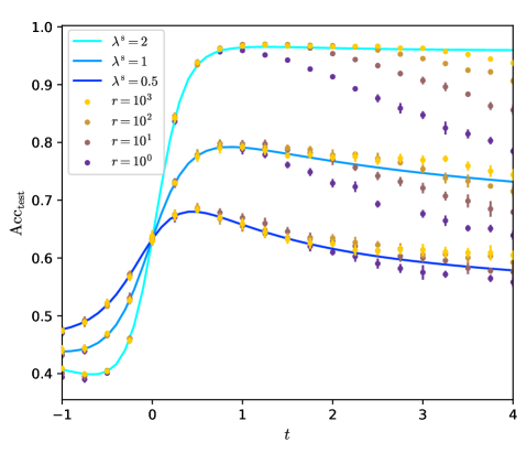
The image is a line chart with error bars, plotting test accuracy (`Acc_test`) against a parameter `t`. It compares the performance of models configured with different values of a regularization or scaling parameter `λ^s` (lambda superscript s) and a parameter `r`. The chart demonstrates how accuracy evolves as `t` increases from -1 to 4 for each configuration.
### Components/Axes
* **X-Axis:** Labeled `t`. Linear scale ranging from -1 to 4, with major tick marks at -1, 0, 1, 2, 3, 4.
* **Y-Axis:** Labeled `Acc_test`. Linear scale ranging from 0.4 to 1.0, with major tick marks at 0.4, 0.5, 0.6, 0.7, 0.8, 0.9, 1.0.
* **Legend (Top-Left Corner):** Contains two distinct groups:
1. **Lines (Solid):** Represent different values of `λ^s`.
* Cyan line: `λ^s = 2`
* Light blue line: `λ^s = 1`
* Dark blue line: `λ^s = 0.5`
2. **Markers (Circles with Error Bars):** Represent different values of `r`.
* Yellow circle: `r = 10^3`
* Gold circle: `r = 10^2`
* Brown circle: `r = 10^1`
* Purple circle: `r = 10^0`
### Detailed Analysis
**Data Series Trends (Lines):**
1. **`λ^s = 2` (Cyan Line):** Shows a steep, sigmoidal increase from `t = -1` (Acc ≈ 0.40) to `t ≈ 0.5`, then plateaus near the maximum accuracy of ~0.97 for `t > 1`. It maintains the highest accuracy across most of the `t` range.
2. **`λ^s = 1` (Light Blue Line):** Increases from `t = -1` (Acc ≈ 0.44) to a peak of ~0.80 at `t ≈ 0.5`, then gradually declines to ~0.73 at `t = 4`.
3. **`λ^s = 0.5` (Dark Blue Line):** Increases from `t = -1` (Acc ≈ 0.48) to a peak of ~0.68 at `t ≈ 0.2`, then declines more steeply to ~0.58 at `t = 4`.
**Data Points by `r` Value (Markers):**
* **General Pattern:** For a given `t` and `λ^s` line, higher `r` values (e.g., `10^3`, yellow) consistently yield higher accuracy points than lower `r` values (e.g., `10^0`, purple). The vertical spread of markers at a given `t` illustrates the impact of `r`.
* **`r = 10^3` (Yellow):** Points cluster very closely to the `λ^s = 2` line, especially for `t > 0`. At `t=4`, accuracy is ~0.97.
* **`r = 10^2` (Gold):** Points generally lie slightly below the `λ^s = 2` line and above the `λ^s = 1` line. At `t=4`, accuracy is ~0.95.
* **`r = 10^1` (Brown):** Points show significant scatter. They are near the `λ^s = 1` line for `t < 1` but fall below it for larger `t`. At `t=4`, accuracy is ~0.82.
* **`r = 10^0` (Purple):** Points exhibit the highest variance and lowest accuracy. They are consistently the lowest set of points. At `t=4`, accuracy is ~0.65.
* **Error Bars:** Vertical error bars are present on all markers, indicating variability in the accuracy measurement. The bars appear larger for lower `r` values (e.g., `r=10^0`, purple) and for points where the trend is changing rapidly (e.g., near `t=0`).
### Key Observations
1. **Dominant Trend:** The `λ^s = 2` configuration achieves the highest and most stable test accuracy for `t > 0.5`.
2. **Parameter Interaction:** The benefit of a higher `r` value is most pronounced for the `λ^s = 2` configuration. For `λ^s = 0.5` and `λ^s = 1`, the performance gap between different `r` values narrows as `t` increases.
3. **Peak and Decline:** Both the `λ^s = 1` and `λ^s = 0.5` series show a clear peak in accuracy at low `t` values (`t ≈ 0.5` and `t ≈ 0.2`, respectively), followed by a decline. This suggests a trade-off or overfitting effect as `t` increases for these configurations.
4. **Convergence at Low `t`:** All lines and most data points converge in the region `t ≈ -0.5` to `t ≈ 0`, with accuracy values between 0.6 and 0.7.
### Interpretation
This chart likely visualizes the results of a machine learning experiment studying the dynamics of model training or generalization. The parameter `t` could represent a training step, a noise scale, or a temperature parameter in a method like diffusion models or stochastic gradient descent.
* **`λ^s` as a Regularizer/Scaler:** A higher `λ^s` (2) appears to act as a strong stabilizing force, enabling the model to reach and maintain high accuracy. Lower values (1, 0.5) lead to an initial improvement followed by degradation, which could indicate instability or overfitting as the process (`t`) continues.
* **`r` as Model Capacity or Data Scale:** The parameter `r` (plotted on a log scale) strongly correlates with performance. Higher `r` (e.g., 1000) likely represents a larger model, more data, or a higher-rank approximation, leading to better and more consistent accuracy. The large error bars for low `r` suggest high sensitivity and instability in low-capacity regimes.
* **The Critical Region:** The most dynamic changes occur between `t = -1` and `t = 1`. This is where configurations diverge, peaks are reached, and the impact of `r` becomes most visually distinct. The post-`t=1` region shows the long-term behavior: stable high performance for `λ^s=2`, and gradual decay for others.
* **Practical Implication:** To achieve robust, high accuracy that persists as `t` increases, the combination of a high `λ^s` (2) and a high `r` (≥100) is optimal. Configurations with lower `λ^s` are only competitive at very specific, low `t` values.