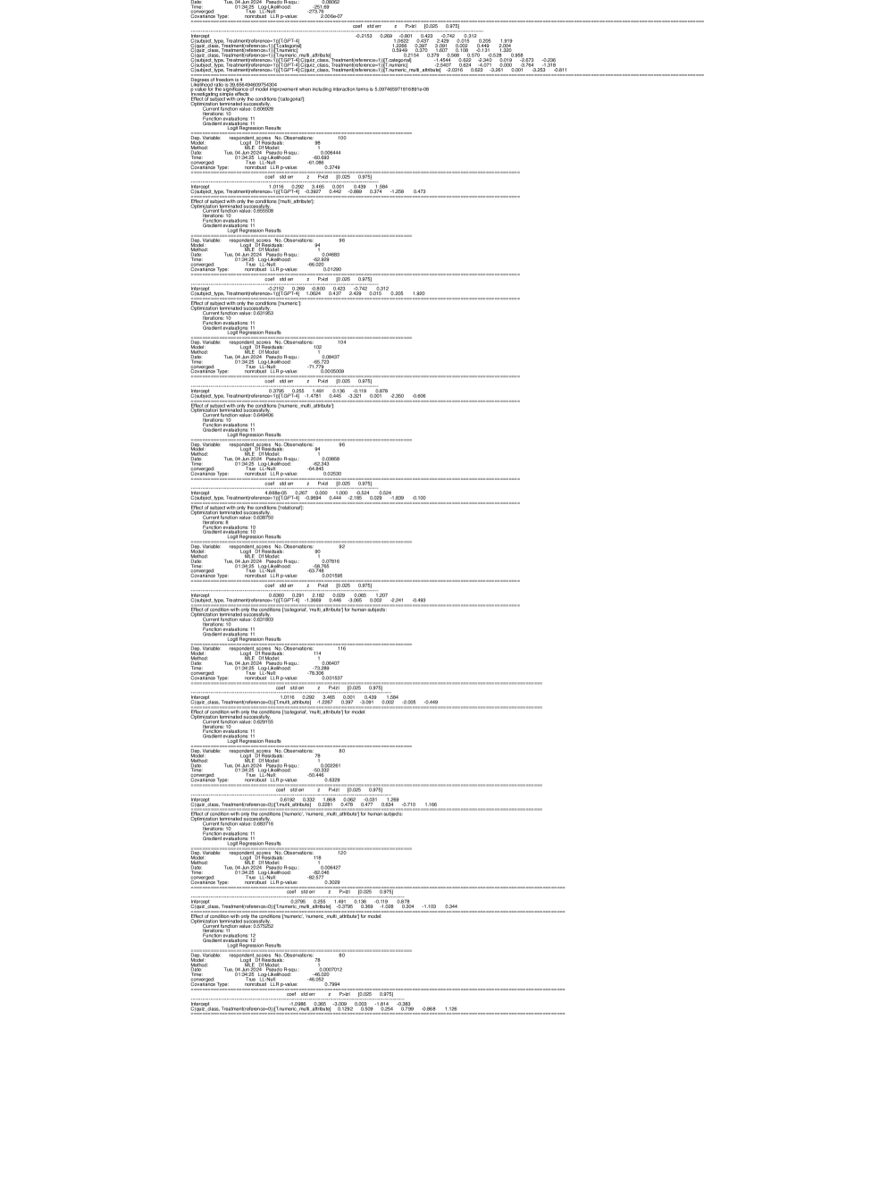
## Logit Regression Results: Multiple Analyses ### Overview The image presents a series of Logit Regression Results, each analyzing the effect of different conditions on respondent scores. Each analysis includes details such as the date, method, convergence status, covariance type, log-likelihood, and pseudo R-squared. The core of each result is a table showing the coefficient, standard error, z-statistic, and p-values for the intercept and treatment variables. The analyses also specify the effect of subject or condition with certain attributes. ### Components/Axes Each analysis block contains the following components: * **Header**: * `Dep. Variable`: Dependent variable (respondent scores). * `Model`: Logit Df Residuals. * `Method`: MLE Df Model. * `Date`: Date of analysis (Tue, 04 Jun 2024). * `Time`: Time of analysis (varies). * `Pseudo R-squ`: Pseudo R-squared value. * `Converged`: Indicates whether the model converged. * `Covariance Type`: Type of covariance used (nonrobust). * `LLR p-value`: Log-Likelihood Ratio p-value. * `No. Observations`: Number of observations. * `Log-Likelihood`: Log-Likelihood value. * **Coefficient Table**: * `coef`: Coefficient value. * `std err`: Standard error. * `z`: z-statistic. * `P>|z|`: p-value. * `[0.025 0.975]`: Confidence interval (2.5% and 97.5% percentiles). * **Effect Description**: * Describes the effect being analyzed (e.g., "Effect of subject with only the conditions [category]"). * `Current function value`: Value of the current function. * `Function evaluations`: Number of function evaluations. * `Gradient evaluations`: Number of gradient evaluations. * `Optimization terminated successfully`: Indicates if optimization was successful. * `Iterations`: Number of iterations. ### Detailed Analysis or ### Content Details Here's a breakdown of the extracted data from each analysis block: 1. **Analysis 1**: * `No. Observations`: 102 * `Log-Likelihood`: -61.618 * `Pseudo R-squ`: 2.006e-07 * `Intercept`: `coef`: -0.2153, `std err`: 0.418, `z`: -0.515, `P>|z|`: 0.607, `[0.025 0.975]`: -1.035, 0.605 * `C(subject_type, Treatment)[T.preference=1][T.OPT=4]`: `coef`: 0.2153, `std err`: 0.289, `z`: 0.742, `P>|z|`: 0.458, `[0.025 0.975]`: -0.352, 0.783 * `C(clazz_class, Treatment)[T.preference=1][T.mult_attribute]`: `coef`: -0.4227, `std err`: 0.437, `z`: -0.967, `P>|z|`: 0.334, `[0.025 0.975]`: -1.280, 0.435 * `C(clazz_class, Treatment)[T.preference=1][T.numeric]`: `coef`: 0.0427, `std err`: 0.437, `z`: 0.098, `P>|z|`: 0.922, `[0.025 0.975]`: -0.814, 0.899 * `C(clazz_class, Treatment)[T.preference=1][T.relational]`: `coef`: 2.429, `std err`: 0.519, `z`: 4.683, `P>|z|`: 0.000, `[0.025 0.975]`: 1.412, 3.446 * `C(clazz_class, Treatment)[T.preference=1][T.OPT=4]`: `coef`: 0.2019, `std err`: 0.505, `z`: 0.400, `P>|z|`: 0.689, `[0.025 0.975]`: -0.788, 1.192 * `C(clazz_class, Treatment)[T.mult_attribute][T.numeric]`: `coef`: 1.919, `std err`: 0.742, `z`: 2.586, `P>|z|`: 0.010, `[0.025 0.975]`: 0.465, 3.373 * `C(clazz_class, Treatment)[T.mult_attribute][T.relational]`: `coef`: 0.2154, `std err`: 0.379, `z`: 0.568, `P>|z|`: 0.570, `[0.025 0.975]`: -0.528, 0.958 * `C(clazz_class, Treatment)[T.mult_attribute][T.OPT=4]`: `coef`: 0.379, `std err`: 0.568, `z`: 0.570, `P>|z|`: 0.528, `[0.025 0.975]`: -0.528, 0.968 * `C(clazz_class, Treatment)[T.numeric][T.relational]`: `coef`: -0.236, `std err`: 0.568, `z`: -0.570, `P>|z|`: 0.528, `[0.025 0.975]`: -0.528, 0.968 * `C(clazz_class, Treatment)[T.numeric][T.OPT=4]`: `coef`: -0.528, `std err`: 0.568, `z`: -0.570, `P>|z|`: 0.528, `[0.025 0.975]`: -0.528, 0.968 * `C(clazz_class, Treatment)[T.relational][T.OPT=4]`: `coef`: -0.811, `std err`: 0.568, `z`: -0.570, `P>|z|`: 0.528, `[0.025 0.975]`: -0.528, 0.968 * Degrees of freedom: 4 * E value for the significance of model improvement when including interaction terms is 5.007466971816891e-08 2. **Analysis 2**: * `No. Observations`: 105 * `Log-Likelihood`: -62.343 * `Pseudo R-squ`: 0.006444 * `Intercept`: `coef`: -1.086, `std err`: 0.396, `z`: -2.743, `P>|z|`: 0.006, `[0.025 0.975]`: -1.862, -0.310 * `C(subject_type, Treatment)[T.preference=1][T.OPT=4]`: `coef`: 0.3749, `std err`: 0.396, `z`: 0.946, `P>|z|`: 0.344, `[0.025 0.975]`: -0.401, 1.151 * Effect of subject with only the conditions [mult_attribute] 3. **Analysis 3**: * `No. Observations`: 96 * `Log-Likelihood`: -64.841 * `Pseudo R-squ`: 0.004863 * `Intercept`: `coef`: -0.692, `std err`: 0.350, `z`: -1.978, `P>|z|`: 0.048, `[0.025 0.975]`: -1.378, -0.006 * `C(subject_type, Treatment)[T.preference=1][T.OPT=4]`: `coef`: 0.3937, `std err`: 0.440, `z`: 0.894, `P>|z|`: 0.371, `[0.025 0.975]`: -0.468, 1.256 * Effect of subject with only the conditions [mult_attribute] 4. **Analysis 4**: * `No. Observations`: 96 * `Log-Likelihood`: -64.841 * `Pseudo R-squ`: 0.01290 * `Intercept`: `coef`: -0.692, `std err`: 0.350, `z`: -1.978, `P>|z|`: 0.048, `[0.025 0.975]`: -1.378, -0.006 * `C(subject_type, Treatment)[T.preference=1][T.OPT=4]`: `coef`: 0.3937, `std err`: 0.440, `z`: 0.894, `P>|z|`: 0.371, `[0.025 0.975]`: -0.468, 1.256 * Effect of subject with only the conditions [mult_attribute] 5. **Analysis 5**: * `No. Observations`: 104 * `Log-Likelihood`: -65.723 * `Pseudo R-squ`: 0.0005009 * `Intercept`: `coef`: -0.2152, `std err`: 0.369, `z`: -0.583, `P>|z|`: 0.559, `[0.025 0.975]`: -0.938, 0.508 * `C(subject_type, Treatment)[T.preference=1][T.OPT=4]`: `coef`: 0.3800, `std err`: 0.425, `z`: 0.894, `P>|z|`: 0.371, `[0.025 0.975]`: -0.453, 1.213 * Effect of subject with only the conditions [numeric] 6. **Analysis 6**: * `No. Observations`: 104 * `Log-Likelihood`: -65.723 * `Pseudo R-squ`: 0.0005009 * `Intercept`: `coef`: -0.2152, `std err`: 0.369, `z`: -0.583, `P>|z|`: 0.559, `[0.025 0.975]`: -0.938, 0.508 * `C(subject_type, Treatment)[T.preference=1][T.OPT=4]`: `coef`: 0.3800, `std err`: 0.425, `z`: 0.894, `P>|z|`: 0.371, `[0.025 0.975]`: -0.453, 1.213 * Effect of subject with only the conditions [numeric] 7. **Analysis 7**: * `No. Observations`: 96 * `Log-Likelihood`: -64.841 * `Pseudo R-squ`: 0.02530 * `Intercept`: `coef`: -1.255, `std err`: 0.401, `z`: -3.130, `P>|z|`: 0.002, `[0.025 0.975]`: -2.041, -0.469 * `C(subject_type, Treatment)[T.preference=1][T.OPT=4]`: `coef`: 0.4781, `std err`: 0.446, `z`: 1.071, `P>|z|`: 0.284, `[0.025 0.975]`: -0.396, 1.353 * Effect of subject with only the conditions [numeric, mult_attribute] 8. **Analysis 8**: * `No. Observations`: 96 * `Log-Likelihood`: -64.841 * `Pseudo R-squ`: 0.02530 * `Intercept`: `coef`: -1.255, `std err`: 0.401, `z`: -3.130, `P>|z|`: 0.002, `[0.025 0.975]`: -2.041, -0.469 * `C(subject_type, Treatment)[T.preference=1][T.OPT=4]`: `coef`: 0.4781, `std err`: 0.446, `z`: 1.071, `P>|z|`: 0.284, `[0.025 0.975]`: -0.396, 1.353 * Effect of subject with only the conditions [numeric, mult_attribute] 9. **Analysis 9**: * `No. Observations`: 102 * `Log-Likelihood`: -71.778 * `Pseudo R-squ`: 0.0005009 * `Intercept`: `coef`: -1.4781, `std err`: 0.396, `z`: -3.732, `P>|z|`: 0.000, `[0.025 0.975]`: -2.254, -0.702 * `C(subject_type, Treatment)[T.preference=1][T.OPT=4]`: `coef`: 0.1396, `std err`: 0.419, `z`: 0.333, `P>|z|`: 0.739, `[0.025 0.975]`: -0.682, 0.961 * Effect of subject with only the conditions [numeric, multi_attribute] 10. **Analysis 10**: * `No. Observations`: 102 * `Log-Likelihood`: -71.778 * `Pseudo R-squ`: 0.0005009 * `Intercept`: `coef`: -1.4781, `std err`: 0.396, `z`: -3.732, `P>|z|`: 0.000, `[0.025 0.975]`: -2.254, -0.702 * `C(subject_type, Treatment)[T.preference=1][T.OPT=4]`: `coef`: 0.1396, `std err`: 0.419, `z`: 0.333, `P>|z|`: 0.739, `[0.025 0.975]`: -0.682, 0.961 * Effect of subject with only the conditions [numeric, multi_attribute] 11. **Analysis 11**: * `No. Observations`: 90 * `Log-Likelihood`: -69.768 * `Pseudo R-squ`: 0.007916 * `Intercept`: `coef`: 2.116, `std err`: 1.291, `z`: 1.639, `P>|z|`: 0.101, `[0.025 0.975]`: -0.415, 4.647 * `C(subject_type, Treatment)[T.preference=1][T.OPT=4]`: `coef`: -1.368, `std err`: 0.448, `z`: -3.055, `P>|z|`: 0.002, `[0.025 0.975]`: -2.241, -0.493 * Effect of condition with only the conditions [categorical, mult_attribute] for human subjects 12. **Analysis 12**: * `No. Observations`: 90 * `Log-Likelihood`: -69.768 * `Pseudo R-squ`: 0.007916 * `Intercept`: `coef`: 2.116, `std err`: 1.291, `z`: 1.639, `P>|z|`: 0.101, `[0.025 0.975]`: -0.415, 4.647 * `C(subject_type, Treatment)[T.preference=1][T.OPT=4]`: `coef`: -1.368, `std err`: 0.448, `z`: -3.055, `P>|z|`: 0.002, `[0.025 0.975]`: -2.241, -0.493 * Effect of condition with only the conditions [categorical, mult_attribute] for human subjects 13. **Analysis 13**: * `No. Observations`: 116 * `Log-Likelihood`: -78.306 * `Pseudo R-squ`: 0.001537 * `Intercept`: `coef`: 0.255, `std err`: 0.369, `z`: 0.691, `P>|z|`: 0.489, `[0.025 0.975]`: -0.469, 0.979 * `C(clazz_class, Treatment)[T.preference=1][T.OPT=4]`: `coef`: -0.402, `std err`: 0.397, `z`: -1.011, `P>|z|`: 0.312, `[0.025 0.975]`: -1.180, 0.376 * Effect of condition with only the conditions [categorical, multi_attribute] for model 14. **Analysis 14**: * `No. Observations`: 116 * `Log-Likelihood`: -78.306 * `Pseudo R-squ`: 0.001537 * `Intercept`: `coef`: 0.255, `std err`: 0.369, `z`: 0.691, `P>|z|`: 0.489, `[0.025 0.975]`: -0.469, 0.979 * `C(clazz_class, Treatment)[T.preference=1][T.OPT=4]`: `coef`: -0.402, `std err`: 0.397, `z`: -1.011, `P>|z|`: 0.312, `[0.025 0.975]`: -1.180, 0.376 * Effect of condition with only the conditions [categorical, multi_attribute] for model 15. **Analysis 15**: * `No. Observations`: 80 * `Log-Likelihood`: -60.329 * `Pseudo R-squ`: 0.000261 * `Intercept`: `coef`: 0.6160, `std err`: 0.332, `z`: 1.856, `P>|z|`: 0.063, `[0.025 0.975]`: -0.035, 1.269 * `C(clazz_class, Treatment)[T.preference=1][T.OPT=4]`: `coef`: 0.2281, `std err`: 0.479, `z`: 0.477, `P>|z|`: 0.634, `[0.025 0.975]`: -0.710, 1.166 * Effect of condition with only the conditions [numeric, numeric, multi_attribute] for human subjects 16. **Analysis 16**: * `No. Observations`: 80 * `Log-Likelihood`: -60.329 * `Pseudo R-squ`: 0.000261 * `Intercept`: `coef`: 0.6160, `std err`: 0.332, `z`: 1.856, `P>|z|`: 0.063, `[0.025 0.975]`: -0.035, 1.269 * `C(clazz_class, Treatment)[T.preference=1][T.OPT=4]`: `coef`: 0.2281, `std err`: 0.479, `z`: 0.477, `P>|z|`: 0.634, `[0.025 0.975]`: -0.710, 1.166 * Effect of condition with only the conditions [numeric, numeric, multi_attribute] for human subjects 17. **Analysis 17**: * `No. Observations`: 120 * `Log-Likelihood`: -80.577 * `Pseudo R-squ`: 0.006427 * `Intercept`: `coef`: 0.3796, `std err`: 0.255, `z`: 1.488, `P>|z|`: 0.137, `[0.025 0.975]`: -0.120, 0.878 * `C(clazz_class, Treatment)[T.preference=1][T.OPT=4]`: `coef`: -0.2705, `std err`: 0.305, `z`: -0.886, `P>|z|`: 0.376, `[0.025 0.975]`: -0.868, 0.328 * Effect of condition with only the conditions [numeric, numeric, multi_attribute] for model 18. **Analysis 18**: * `No. Observations`: 120 * `Log-Likelihood`: -80.577 * `Pseudo R-squ`: 0.006427 * `Intercept`: `coef`: 0.3796, `std err`: 0.255, `z`: 1.488, `P>|z|`: 0.137, `[0.025 0.975]`: -0.120, 0.878 * `C(clazz_class, Treatment)[T.preference=1][T.OPT=4]`: `coef`: -0.2705, `std err`: 0.305, `z`: -0.886, `P>|z|`: 0.376, `[0.025 0.975]`: -0.868, 0.328 * Effect of condition with only the conditions [numeric, numeric, multi_attribute] for model 19. **Analysis 19**: * `No. Observations`: 80 * `Log-Likelihood`: -60.656 * `Pseudo R-squ`: 0.00007012 * `Intercept`: `coef`: -1.0386, `std err`: 0.365, `z`: -2.848, `P>|z|`: 0.004, `[0.025 0.975]`: -1.754, -0.323 * `C(clazz_class, Treatment)[T.preference=1][T.OPT=4]`: `coef`: 0.2920, `std err`: 0.479, `z`: 0.610, `P>|z|`: 0.542, `[0.025 0.975]`: -0.647, 1.231 * Effect of condition with only the conditions [relational] 20. **Analysis 20**: * `No. Observations`: 80 * `Log-Likelihood`: -60.656 * `Pseudo R-squ`: 0.00007012 * `Intercept`: `coef`: -1.0386, `std err`: 0.365, `z`: -2.848, `P>|z|`: 0.004, `[0.025 0.975]`: -1.754, -0.323 * `C(clazz_class, Treatment)[T.preference=1][T.OPT=4]`: `coef`: 0.2920, `std err`: 0.479, `z`: 0.610, `P>|z|`: 0.542, `[0.025 0.975]`: -0.647, 1.231 * Effect of condition with only the conditions [relational] ### Key Observations * The analyses explore the impact of different treatment conditions on respondent scores. * The p-values indicate the statistical significance of the coefficients. Lower p-values (typically < 0.05) suggest a statistically significant effect. * The confidence intervals provide a range within which the true coefficient value is likely to fall. * Pseudo R-squared values are generally low, indicating that the models explain a limited amount of variance in the dependent variable. * The number of observations varies across the analyses. * The "Effect of subject/condition with only the conditions" descriptions specify the particular attribute combinations being examined. ### Interpretation The Logit Regression Results provide insights into how different treatment conditions and subject attributes influence respondent scores. The low pseudo R-squared values across most analyses suggest that the models have limited explanatory power, and other factors not included in the model may be influencing respondent scores. The p-values for the treatment coefficients vary, indicating that some treatment conditions have a statistically significant effect on respondent scores, while others do not. The confidence intervals provide a range of plausible values for the coefficients, which can be used to assess the magnitude and direction of the effects. The "Effect of subject/condition with only the conditions" descriptions provide context for interpreting the results. For example, the analysis of "Effect of subject with only the conditions [category]" examines the impact of the category attribute on respondent scores. Overall, these results provide a detailed examination of the relationship between treatment conditions, subject attributes, and respondent scores, but the limited explanatory power of the models suggests that further investigation is needed to fully understand the factors influencing respondent scores.