## Dual-Panel Performance Analysis: CIM-SFC vs. NMFA
### Overview
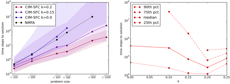
The image contains two side-by-side line charts analyzing the performance of an algorithm or method called "CIM-SFC" with varying parameter `k`, compared to a baseline method "NMFA". The charts plot "time steps to solution" against "problem size" (left) and the parameter `k` (right). Both charts use a logarithmic scale for the y-axis.
### Components/Axes
**Left Chart:**
* **Title:** None visible.
* **X-axis:** Label: `problem size`. Ticks: `√100`, `√200`, `√400`, `√500`, `√800`, `√1000`. This suggests the problem size is the square root of the labeled value (e.g., size 10, ~14.14, 20, ~22.36, ~28.28, ~31.62).
* **Y-axis:** Label: `time steps to solution`. Scale: Logarithmic, from `10^4` to `10^8`.
* **Legend (Top-Left):** Contains four entries:
1. `CIM-SFC k=0.2` (Red line, solid circle markers)
2. `CIM-SFC k=0.15` (Purple line, solid circle markers)
3. `CIM-SFC k=0.0` (Blue line, solid circle markers)
4. `NMFA` (Black dashed line, solid circle markers)
* **Data Series:** Each line has shaded regions (matching line color) representing confidence intervals or variance.
**Right Chart:**
* **Title:** None visible.
* **X-axis:** Label: `k`. Ticks: `0.00`, `0.05`, `0.10`, `0.15`, `0.20`, `0.25`.
* **Y-axis:** Label: `time steps to solution`. Scale: Logarithmic, from `10^4` to `10^8`.
* **Legend (Top-Right):** Contains four entries:
1. `90th pct` (Red dashed line, solid circle markers)
2. `75th pct` (Red dash-dot line, solid circle markers)
3. `median` (Red solid line, solid circle markers)
4. `25th pct` (Red dotted line, solid circle markers)
* **Data Series:** All lines are shades of red, differentiated by line style. They appear to represent the distribution of `time steps to solution` for the CIM-SFC method as a function of `k`.
### Detailed Analysis
**Left Chart - Scaling with Problem Size:**
* **Trend Verification:** All four lines show a clear upward trend, indicating that time steps to solution increase with problem size. The relationship appears roughly linear on this log-log plot, suggesting a polynomial time complexity.
* **Data Points (Approximate from visual inspection):**
* **CIM-SFC k=0.2 (Red):** The lowest line. At `√100`: ~4x10^4. At `√1000`: ~4x10^5.
* **CIM-SFC k=0.15 (Purple):** Middle line. At `√100`: ~5x10^4. At `√1000`: ~2x10^6.
* **CIM-SFC k=0.0 (Blue):** Highest of the CIM-SFC lines. At `√100`: ~6x10^4. At `√500`: ~2x10^6. (Data stops at √500).
* **NMFA (Black Dashed):** The highest line overall. At `√100`: ~7x10^4. At `√800`: ~1x10^7.
* **Spatial Grounding:** The legend is positioned in the top-left corner of the plot area. The shaded confidence intervals are widest for the NMFA and CIM-SFC k=0.0 series, indicating higher variance in their performance.
**Right Chart - Effect of Parameter k:**
* **Trend Verification:** The lines show a non-monotonic relationship with `k`. Time steps generally decrease from `k=0.00` to a minimum around `k=0.15` to `k=0.20`, then increase again at `k=0.25`.
* **Data Points (Approximate):**
* **90th pct (Red Dashed):** Highest values. Starts at `k=0.00`: ~4x10^5. Minimum at `k=0.20`: ~2x10^5. Rises at `k=0.25`: ~3x10^5.
* **75th pct (Red Dash-Dot):** Starts at `k=0.00`: ~3x10^5. Minimum at `k=0.20`: ~8x10^4. Rises at `k=0.25`: ~1x10^5.
* **median (Red Solid):** Starts at `k=0.00`: ~4x10^4. Minimum at `k=0.20`: ~3x10^4. Rises at `k=0.25`: ~8x10^4.
* **25th pct (Red Dotted):** Lowest values. Starts at `k=0.00`: ~6x10^3. Minimum at `k=0.15`: ~1x10^3. Rises at `k=0.25`: ~4x10^3.
* **Spatial Grounding:** The legend is positioned in the top-right corner of the plot area. The spread between the 90th and 25th percentiles is largest at `k=0.00` and narrows significantly around the optimal `k` range (`0.15-0.20`).
### Key Observations
1. **Clear Performance Hierarchy:** For all problem sizes, `CIM-SFC k=0.2` is the fastest, followed by `k=0.15`, then `k=0.0`. The baseline `NMFA` is consistently the slowest.
2. **Optimal k Value:** The right chart strongly suggests an optimal value for parameter `k` exists between 0.15 and 0.20, where the median time steps are minimized and the variance (spread between percentiles) is also reduced.
3. **Scaling Behavior:** The left chart shows that the performance advantage of `CIM-SFC` (especially with tuned `k`) over `NMFA` grows as the problem size increases. The gap between the lines widens on the log scale.
4. **Variance Insight:** The wide confidence intervals in the left chart and the large percentile spread in the right chart (especially at `k=0.00`) indicate that algorithm performance can be highly variable, but this variability is reduced at the optimal `k`.
### Interpretation
This data demonstrates the effectiveness of the `CIM-SFC` method and the critical importance of tuning its `k` parameter. The left chart provides a **Peircean abductive inference**: the consistent ordering of the lines suggests that `k` controls a trade-off, likely between exploration and exploitation or solution quality and speed. A higher `k` (0.2) yields faster solutions, but the right chart reveals this comes at the cost of higher variance (wider percentile spread) at extreme `k` values.
The right chart is a **parameter sensitivity analysis**. The "U-shaped" curve for all percentiles is a classic signature of an optimization landscape, indicating that `k=0` (perhaps meaning no use of a specific heuristic or resource) is suboptimal, and over-tuning (`k=0.25`) also degrades performance. The narrowing of the percentile band at the optimum suggests the algorithm becomes more **robust and predictable** when properly configured.
**Notable Anomaly:** The `CIM-SFC k=0.0` line (blue) in the left chart stops at problem size `√500`, while others continue. This could indicate a failure to converge, a timeout, or simply missing data for larger sizes with that parameter setting, which itself is a significant finding about the limits of that configuration.