## Chart: Time Steps to Solution vs. Problem Size and k-value
### Overview
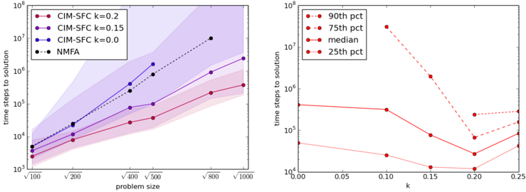
The image presents two line charts comparing the performance of different algorithms in terms of "time steps to solution." The left chart shows the relationship between "time steps to solution" and "problem size" for CIM-SFC with varying k-values (0.2, 0.15, 0.0) and NMFA. The right chart shows the relationship between "time steps to solution" and "k" for the 90th, 75th, median, and 25th percentiles. Both charts use a logarithmic scale for the y-axis ("time steps to solution").
### Components/Axes
**Left Chart:**
* **X-axis:** "problem size" with markers at approximately √100, √200, √400, √500, √800, and √1000.
* **Y-axis:** "time steps to solution" (logarithmic scale) with markers at 10^3, 10^4, 10^5, 10^6, 10^7, and 10^8.
* **Legend (top-left):**
* Red: CIM-SFC k=0.2
* Purple: CIM-SFC k=0.15
* Blue: CIM-SFC k=0.0
* Black: NMFA
**Right Chart:**
* **X-axis:** "k" with markers at 0.00, 0.05, 0.10, 0.15, 0.20, and 0.25.
* **Y-axis:** "time steps to solution" (logarithmic scale) with markers at 10^4, 10^5, 10^6, 10^7, and 10^8.
* **Legend (top-left):**
* Red dotted: 90th pct
* Red dashed: 75th pct
* Red solid: median
* Red dotted: 25th pct
### Detailed Analysis
**Left Chart:**
* **CIM-SFC k=0.2 (Red):** The line slopes upward.
* √100: ~4 x 10^3
* √200: ~9 x 10^3
* √400: ~3 x 10^4
* √500: ~5 x 10^4
* √800: ~1.5 x 10^5
* √1000: ~2 x 10^5
* **CIM-SFC k=0.15 (Purple):** The line slopes upward.
* √100: ~4 x 10^3
* √200: ~1.5 x 10^4
* √400: ~8 x 10^4
* √500: ~1 x 10^5
* √800: ~5 x 10^6
* √1000: ~8 x 10^6
* **CIM-SFC k=0.0 (Blue):** The line slopes upward.
* √100: ~4 x 10^3
* √200: ~2 x 10^4
* √400: ~1 x 10^5
* √500: ~2 x 10^5
* **NMFA (Black, dotted):** The line slopes upward.
* √100: ~4 x 10^3
* √200: ~2.5 x 10^4
* √400: ~2 x 10^5
* √500: ~4 x 10^5
* √800: ~1 x 10^7
**Right Chart:**
* **90th pct (Red, dotted):** The line decreases until k=0.2, then increases.
* 0.00: ~5 x 10^7
* 0.05: ~4 x 10^7
* 0.10: ~2 x 10^7
* 0.15: ~4 x 10^6
* 0.20: ~2 x 10^6
* 0.25: ~4 x 10^6
* **75th pct (Red, dashed):** The line decreases until k=0.2, then increases.
* 0.00: ~5 x 10^6
* 0.05: ~4 x 10^6
* 0.10: ~2 x 10^6
* 0.15: ~4 x 10^5
* 0.20: ~2 x 10^5
* 0.25: ~4 x 10^5
* **Median (Red, solid):** The line decreases until k=0.2, then increases.
* 0.00: ~5 x 10^5
* 0.05: ~4 x 10^5
* 0.10: ~2 x 10^5
* 0.15: ~4 x 10^4
* 0.20: ~2 x 10^4
* 0.25: ~4 x 10^4
* **25th pct (Red, dotted):** The line decreases until k=0.2, then increases.
* 0.00: ~2.5 x 10^4
* 0.05: ~2 x 10^4
* 0.10: ~1 x 10^4
* 0.15: ~2 x 10^3
* 0.20: ~1 x 10^3
* 0.25: ~2 x 10^3
### Key Observations
* In the left chart, for a given problem size, NMFA generally requires more time steps to solution than CIM-SFC with different k values.
* In the left chart, as the problem size increases, the time steps to solution also increase for all algorithms.
* In the right chart, the time steps to solution generally decrease as 'k' increases from 0.00 to 0.20, and then increase as 'k' increases from 0.20 to 0.25 for all percentiles.
* The right chart shows a clear trend of decreasing time steps to solution with increasing 'k' up to a point, suggesting an optimal 'k' value around 0.20.
### Interpretation
The charts suggest that CIM-SFC algorithms are more efficient than NMFA for the tested problem sizes. The optimal 'k' value for minimizing the time steps to solution appears to be around 0.20. The performance of all algorithms degrades as the problem size increases, which is expected. The percentile data in the right chart indicates the distribution of time steps to solution for different 'k' values, with the median representing the typical performance and the 25th and 75th percentiles indicating the range of variability. The 90th percentile shows the worst-case performance.