## Line Chart: Generalization Error vs. Optimization Steps
### Overview
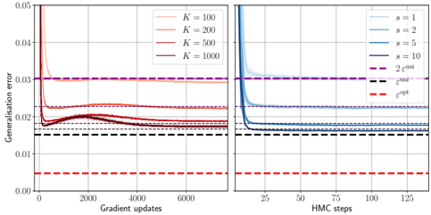
The image displays two side-by-side line charts comparing the generalization error of a model during two different optimization processes: gradient updates (left panel) and Hamiltonian Monte Carlo (HMC) steps (right panel). Each chart plots multiple data series corresponding to different hyperparameter values (`K` and `s`), alongside several constant baseline error levels.
### Components/Axes
**Common Y-Axis (Both Panels):**
* **Label:** `Generalization error`
* **Scale:** Linear, ranging from `0.00` to `0.05`. Major ticks at intervals of `0.01`.
**Left Panel X-Axis:**
* **Label:** `Gradient updates`
* **Scale:** Linear, ranging from `0` to `6000`. Major ticks at `0, 2000, 4000, 6000`.
**Right Panel X-Axis:**
* **Label:** `HMC steps`
* **Scale:** Linear, ranging from `0` to `125`. Major ticks at `0, 25, 50, 75, 100, 125`.
**Legends & Baselines:**
* **Left Panel Legend (Top-Right):** Four solid lines in shades of red/orange, labeled:
* `K = 100` (lightest orange)
* `K = 200`
* `K = 500`
* `K = 1000` (darkest red)
* **Right Panel Legend (Top-Right):** Four solid lines in shades of blue, labeled:
* `s = 1` (lightest blue)
* `s = 2`
* `s = 5`
* `s = 10` (darkest blue)
* **Horizontal Dashed Baselines (Present in both panels):**
* `2ε^noise` (Magenta/Purple dashed line) at approximately `y = 0.030`.
* `ε^train` (Black dashed line) at approximately `y = 0.015`.
* `ε^opt` (Red dashed line) at approximately `y = 0.005`.
### Detailed Analysis
**Left Panel: Gradient Updates**
* **Trend Verification:** All four `K` series follow a similar pattern: a very steep initial drop in generalization error within the first few hundred updates, followed by a rapid plateau. The lines remain largely flat after ~1000 updates.
* **Data Points & Relationships:**
* The series for `K=100` (light orange) plateaus at the highest error level, just above the `ε^train` baseline (~0.016).
* The series for `K=200` (medium orange) plateaus slightly lower, very close to the `ε^train` line.
* The series for `K=500` (dark orange) and `K=1000` (dark red) plateau at the lowest levels among the `K` series, settling between the `ε^train` and `ε^opt` baselines (approximately 0.013-0.014). The `K=1000` line appears marginally lower than the `K=500` line.
* All `K` series remain significantly above the `ε^opt` baseline and below the `2ε^noise` baseline throughout.
**Right Panel: HMC Steps**
* **Trend Verification:** All four `s` series exhibit an extremely sharp, near-vertical drop in error within the first 5-10 HMC steps, followed by an immediate and stable plateau for the remainder of the steps shown.
* **Data Points & Relationships:**
* The series for `s=1` (light blue) plateaus at the highest error level, slightly above the `ε^train` baseline (~0.016).
* The series for `s=2` (medium blue) plateaus just below the `ε^train` line.
* The series for `s=5` (dark blue) and `s=10` (darkest blue) plateau at the lowest levels, settling very close to each other and just above the `ε^opt` baseline (approximately 0.006-0.007). The `s=10` line is visually indistinguishable from or marginally lower than the `s=5` line.
* All `s` series remain below the `2ε^noise` baseline. The higher `s` values (`5` and `10`) come very close to the `ε^opt` baseline.
### Key Observations
1. **Convergence Speed:** Both optimization methods show extremely rapid initial convergence. HMC (right panel) appears to reach its plateau in far fewer steps (first ~10 steps) compared to gradient updates (first ~500-1000 updates).
2. **Hyperparameter Impact:** Increasing the hyperparameter (`K` for gradient updates, `s` for HMC) consistently leads to a lower final generalization error plateau.
3. **Performance Relative to Baselines:** The HMC method, particularly with higher `s` values (`s=5, 10`), achieves a final generalization error that is much closer to the theoretical optimum (`ε^opt`) than the gradient update method does with any `K` value shown.
4. **Plateau Stability:** After the initial drop, all curves are remarkably flat, indicating no further improvement (or degradation) in generalization error with additional optimization steps within the ranges plotted.
### Interpretation
This data suggests a comparative study of optimization algorithms for a machine learning model. The `Generalization error` is the key performance metric.
* **What the data demonstrates:** The charts argue that the HMC optimization method (right panel) is more sample-efficient and effective at minimizing generalization error than standard gradient updates (left panel) for this specific task. It reaches a better final solution (closer to `ε^opt`) in dramatically fewer steps.
* **Relationship between elements:** The hyperparameters `K` and `s` likely control aspects like ensemble size or sampling depth. Their positive correlation with performance (higher value → lower error) indicates that increased computational budget or model complexity within each method yields better results, but with diminishing returns (the gap between `K=500` and `K=1000` is smaller than between `K=100` and `K=200`).
* **Notable Anomalies/Insights:** The most striking insight is the stark difference in convergence profiles. The near-instantaneous plateau of HMC suggests it may be navigating the loss landscape more effectively, perhaps by avoiding poor local minima that gradient descent might linger in. The fact that even the best HMC result (`s=10`) does not reach the `ε^opt` line indicates there is still a gap between the achieved performance and the theoretical optimum, possibly due to model limitations or noise in the data (`2ε^noise`). The consistent ordering of the baselines (`ε^opt` < `ε^train` < `2ε^noise`) provides a crucial frame of reference for evaluating the absolute performance of each method.