## Line Graphs: Generalization Error vs. Optimization Steps
### Overview
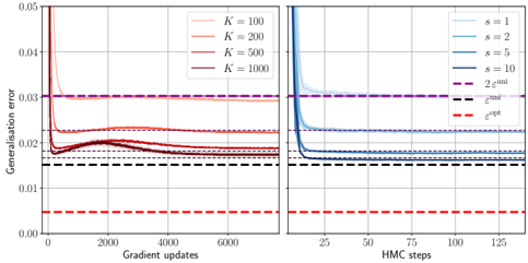
The image contains two side-by-side line graphs comparing generalization error trends across different optimization parameters. The left graph tracks generalization error against gradient updates, while the right graph tracks it against Hamiltonian Monte Carlo (HMC) steps. Both graphs include convergence bounds (ε_uni and ε_opt) and show distinct performance patterns for varying parameter configurations.
### Components/Axes
**Left Graph (Gradient Updates):**
- **X-axis**: Gradient updates (0–6000, linear scale)
- **Y-axis**: Generalisation error (0.00–0.05, linear scale)
- **Legend**:
- Solid lines: K=100 (orange), K=200 (red), K=500 (dark red), K=1000 (purple)
- Dashed lines: ε_uni (black), ε_opt (red)
- **Key Elements**:
- Purple dashed line at y=0.03 (ε_uni)
- Red dashed line at y=0.01 (ε_opt)
**Right Graph (HMC Steps):**
- **X-axis**: HMC steps (0–125, linear scale)
- **Y-axis**: Generalisation error (same scale as left graph)
- **Legend**:
- Solid lines: s=1 (light blue), s=2 (medium blue), s=5 (dark blue), s=10 (very dark blue)
- Dashed lines: ε_uni (black), ε_opt (red)
- **Key Elements**:
- Same ε_uni and ε_opt bounds as left graph
### Detailed Analysis
**Left Graph Trends:**
1. **K=100 (orange)**: Sharp initial drop to ~0.025 at 1000 updates, then gradual decline to ~0.018 by 6000 updates.
2. **K=200 (red)**: Steeper initial decline to ~0.02 at 1000 updates, plateauing near ε_opt (~0.01) by 4000 updates.
3. **K=500 (dark red)**: Rapid convergence to ~0.015 by 2000 updates, maintaining near ε_opt.
4. **K=1000 (purple)**: Fastest convergence, reaching ε_opt (~0.01) by 1000 updates and staying flat.
**Right Graph Trends:**
1. **s=1 (light blue)**: Gradual decline from 0.04 to ~0.02 over 100 steps, then slow improvement.
2. **s=2 (medium blue)**: Faster initial drop to ~0.025 by 50 steps, then plateau.
3. **s=5 (dark blue)**: Sharp decline to ~0.015 by 75 steps, maintaining near ε_opt.
4. **s=10 (very dark blue)**: Most efficient, reaching ε_opt (~0.01) by 50 steps and stabilizing.
### Key Observations
1. **Convergence Patterns**:
- Higher K/s values achieve lower generalization error faster.
- Both methods converge toward ε_opt, but HMC steps (right graph) show sharper initial declines.
2. **Bound Relationships**:
- ε_opt (red dashed line) is consistently ~3× lower than ε_uni (black dashed line), indicating tighter optimization bounds.
3. **Parameter Sensitivity**:
- K=1000 and s=10 outperform all other configurations, suggesting diminishing returns beyond these thresholds.
### Interpretation
The graphs demonstrate that both gradient updates and HMC steps reduce generalization error, with parameter scaling (K/s) being critical. The ε_opt bound represents an idealized minimum error, while ε_uni reflects a looser theoretical limit. The right graph's HMC method achieves lower error faster for high s values, suggesting it may be more sample-efficient than gradient descent for this task. The left graph's slower convergence for lower K values highlights the importance of batch size in stochastic optimization. The consistent gap between ε_opt and ε_uni across both graphs implies that the optimization landscape has inherent structural constraints that prevent reaching the theoretical minimum error.