# Technical Document Extraction: Decision Tree and Feature Space Partitioning
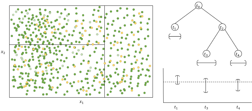
This image illustrates the relationship between a partitioned 2D feature space, a corresponding decision tree structure, and the resulting leaf node predictions.
## 1. Component Isolation
The image is divided into three primary functional regions:
* **Left Region (Feature Space Plot):** A 2D scatter plot showing data points and recursive partitioning.
* **Top-Right Region (Decision Tree Diagram):** A hierarchical tree structure representing the logic used to partition the feature space.
* **Bottom-Right Region (Prediction Plot):** A visualization of the values or intervals associated with the terminal (leaf) nodes of the tree.
---
## 2. Feature Space Plot (Left)
This region represents a two-dimensional feature space defined by axes $x_1$ and $x_2$.
### Axis Labels
* **X-axis:** $x_1$ (Horizontal)
* **Y-axis:** $x_2$ (Vertical)
### Data Points
The plot contains a high density of scatter points in two distinct colors:
* **Green Points:** Predominant throughout the space.
* **Yellow/Gold Points:** Interspersed among the green points, appearing as a secondary class or value.
* **Note:** Some points appear with lower opacity (faded), possibly indicating historical data or points outside a specific weight threshold.
### Partitioning (Spatial Grounding)
The space is divided into three distinct rectangular regions by solid black lines:
1. **Right Vertical Partition:** A vertical line at a specific $x_1$ value separates the rightmost section of the plot.
2. **Left Horizontal Partition:** A horizontal line at a specific $x_2$ value divides the remaining left area into an upper-left and a lower-left quadrant.
---
## 3. Decision Tree Diagram (Top-Right)
This diagram maps the logic of the partitions shown in the Feature Space Plot.
### Nodes and Hierarchy
* **Root Node ($t_0$):** The top-level node representing the first split.
* **Left Branch:** Leads to leaf node **$t_1$**.
* **Right Branch:** Leads to internal node **$t_2$**.
* **Internal Node ($t_2$):** Represents the second split.
* **Left Branch:** Leads to leaf node **$t_3$**.
* **Right Branch:** Leads to leaf node **$t_4$**.
### Terminal Nodes (Leaf Nodes)
The leaf nodes are identified as:
* **$t_1$**: Corresponds to the right-hand vertical partition in the feature space.
* **$t_3$**: Corresponds to one of the horizontal sub-partitions on the left.
* **$t_4$**: Corresponds to the other horizontal sub-partition on the left.
Below each leaf node ($t_1, t_3, t_4$), there is a horizontal bracket symbol `[—]` indicating a range or interval associated with that node.
---
## 4. Prediction Plot (Bottom-Right)
This chart visualizes the output or "prediction" associated with each leaf node.
### Axis and Markers
* **X-axis Labels:** $t_1$, $t_3$, $t_4$ (corresponding to the tree's leaf nodes).
* **Y-axis:** Unlabeled vertical axis representing a continuous value.
* **Baseline:** A horizontal dashed line runs across the plot, representing a global mean or a reference threshold.
### Data Series: Prediction Intervals
For each leaf node, a vertical error bar (I-beam) is plotted:
* **$t_1$ Trend:** The interval is centered slightly above the dashed baseline.
* **$t_3$ Trend:** The interval is significantly larger and centered below the dashed baseline.
* **$t_4$ Trend:** The interval is centered slightly above the dashed baseline, similar to $t_1$ but with a slightly different vertical span.
---
## 5. Summary of Logic and Flow
1. **Input:** Data points are distributed in a 2D space ($x_1, x_2$).
2. **Process:** A decision tree performs recursive binary splitting.
* The first split at $t_0$ isolates the right-hand region ($t_1$).
* The second split at $t_2$ divides the remaining left-hand region into $t_3$ and $t_4$.
3. **Output:** Each resulting region (leaf node) is assigned a predictive value and an uncertainty interval, as shown in the bottom-right graph. $t_3$ shows the highest variance/interval range compared to $t_1$ and $t_4$.