## Diagram: Comparison of Proof Strategies With and Without Backtracking
### Overview
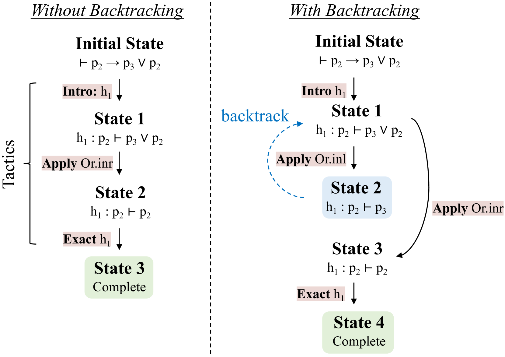
The image is a technical diagram comparing two approaches to constructing a formal logical proof: one that proceeds linearly without backtracking and one that incorporates a backtracking step to explore an alternative path. The diagram is split vertically by a dashed line, with the left side titled "Without Backtracking" and the right side titled "With Backtracking". Both sides begin with the same initial logical statement and use a series of "Tactics" to reach a "Complete" state.
### Components/Axes
The diagram is a flowchart-style state transition diagram. There are no traditional chart axes. The key components are:
* **Titles:** "Without Backtracking" (top left), "With Backtracking" (top right).
* **States:** Represented by text blocks, often with a label (e.g., "Initial State", "State 1") and a logical sequent.
* **Tactics:** Represented by text in pinkish-red boxes (e.g., "Intro: h₁", "Apply Or.inr"). These are the actions that transform one state into the next.
* **Arrows:** Solid black arrows indicate the forward progression of the proof. A dashed blue arrow labeled "backtrack" indicates a return to a previous state to try a different tactic.
* **Completion Indicator:** A green box labeled "Complete" signifies the end of a successful proof.
* **Grouping Label:** A bracket on the left side groups the tactics under the label "Tactics".
### Detailed Analysis
The proof attempts to demonstrate the logical theorem: `⊢ p₂ → p₃ ∨ p₂`.
**Left Side: Without Backtracking**
1. **Initial State:** `⊢ p₂ → p₃ ∨ p₂`
2. **Tactic Applied:** `Intro: h₁` (Introduces hypothesis `h₁: p₂`).
3. **State 1:** `h₁ : p₂ ⊢ p₃ ∨ p₂`
4. **Tactic Applied:** `Apply Or.inr` (Chooses to prove the right disjunct, `p₂`).
5. **State 2:** `h₁ : p₂ ⊢ p₂`
6. **Tactic Applied:** `Exact h₁` (Uses hypothesis `h₁` directly to close the goal).
7. **State 3 / Complete:** The proof is successfully finished.
**Right Side: With Backtracking**
1. **Initial State:** `⊢ p₂ → p₃ ∨ p₂` (Identical to left side).
2. **Tactic Applied:** `Intro h₁` (Identical to left side).
3. **State 1:** `h₁ : p₂ ⊢ p₃ ∨ p₂` (Identical to left side).
4. **First Tactic Attempt:** `Apply Or.inl` (Chooses to prove the left disjunct, `p₃`).
5. **State 2:** `h₁ : p₂ ⊢ p₃` (This state is highlighted with a light blue background, indicating it is a dead end or problematic path).
6. **Backtrack Action:** A dashed blue arrow labeled "backtrack" curves from State 2 back to State 1. This indicates the proof engine abandons the `Apply Or.inl` path.
7. **Alternative Tactic Applied:** From State 1, the tactic `Apply Or.inr` is now applied (this is the same tactic that was used directly on the left side).
8. **State 3:** `h₁ : p₂ ⊢ p₂` (This matches State 2 from the left-side proof).
9. **Tactic Applied:** `Exact h₁`.
10. **State 4 / Complete:** The proof is successfully finished.
### Key Observations
* **Identical Starting Point:** Both proofs begin with the same goal and initial tactic (`Intro`).
* **Divergent First Choice:** The critical difference is the first choice of disjunction elimination tactic. The left side correctly chooses `Or.inr` immediately. The right side first attempts `Or.inl`, which leads to an unprovable state (`⊢ p₃`).
* **Backtracking Mechanism:** The right side explicitly models the process of recognizing a failed path (`State 2`), returning to the decision point (`State 1`), and trying the alternative (`Or.inr`).
* **Outcome:** Both strategies ultimately succeed, but the backtracking strategy involves an extra, failed step. The "Without Backtracking" path is more efficient.
* **Visual Coding:** The use of a blue highlight on the dead-end state and a blue dashed arrow for the backtrack action clearly distinguishes the exploratory, non-linear nature of the right-side process.
### Interpretation
This diagram illustrates a fundamental concept in automated theorem proving and interactive proof assistants: **proof search strategy**.
* **What it demonstrates:** It shows that for a given goal, there may be multiple applicable tactics (here, `Or.inl` and `Or.inr` for proving a disjunction). A naive or uninformed search might try an incorrect path first.
* **The role of backtracking:** Backtracking is a control mechanism that allows a proof search to recover from poor tactical choices. It enables exhaustive exploration of the proof space by systematically trying alternatives when a path fails. The diagram visually argues that while backtracking guarantees finding a proof if one exists (given enough time and resources), a more intelligent or heuristic-driven strategy (like the one on the left that picks the correct tactic first) is more efficient.
* **Underlying logic:** The specific theorem `p₂ → p₃ ∨ p₂` is a tautology. The proof hinges on the fact that if `p₂` is true, then the disjunction `p₃ ∨ p₂` is true regardless of `p₃`. The tactic `Or.inr` exploits this by focusing on proving `p₂`, which is directly available from the hypothesis. The failed `Or.inl` path attempts to prove `p₃`, which is not supported by the available hypotheses (`h₁: p₂`), hence the dead end.
* **Broader context:** This is a microcosm of how complex proofs are built. In larger proofs, the search space is vast, and the choice of tactics, along with the ability to backtrack, becomes crucial for automation and user-guided proof development. The diagram serves as a clear pedagogical tool for explaining this core concept.