\n
## Diagram: Proof State Transition with and without Backtracking
### Overview
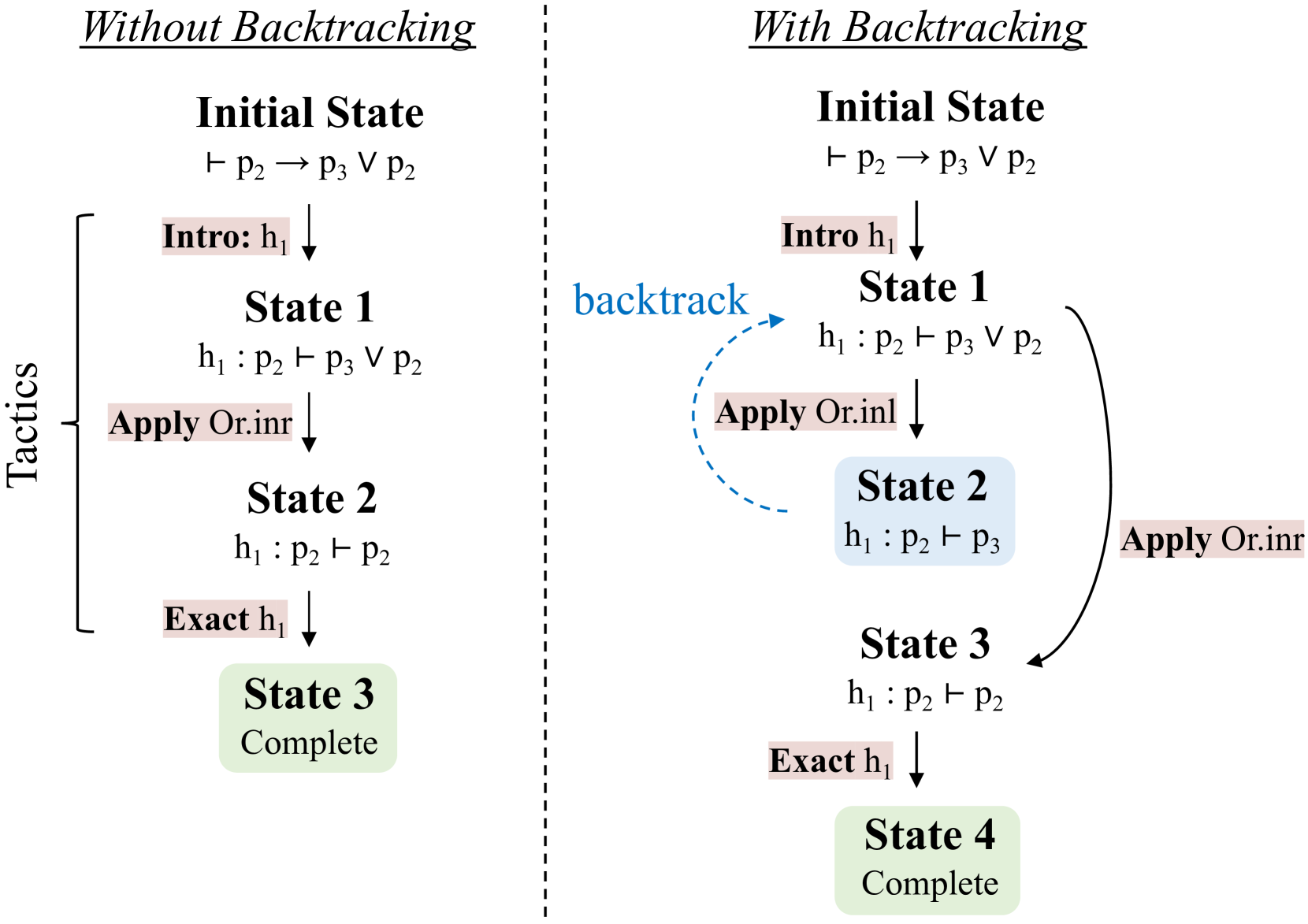
The image presents a comparative diagram illustrating proof state transitions in a logical system, with and without backtracking. The left side demonstrates the process *without* backtracking, while the right side shows the process *with* backtracking. Both sides depict a sequence of states, labeled "Initial State," "State 1," "State 2," and "State 3" (and "State 4" on the right side), connected by arrows representing the application of tactics. A vertical dashed line separates the two scenarios. The left side has a label "Tactics" on the left edge.
### Components/Axes
The diagram consists of:
* **States:** Represented by rounded rectangles labeled "Initial State," "State 1," "State 2," "State 3," and "State 4."
* **Tactics:** Represented by text labels along the arrows connecting the states (e.g., "Intro h₁", "Apply Or.inr", "Exact h₁").
* **Arrows:** Indicate the flow of the proof process. A dashed, curved arrow labeled "backtrack" is present on the right side.
* **Labels:** "Without Backtracking" and "With Backtracking" are used to title the two sections.
* **Logical Statements:** Each state contains a logical statement of the form "Γ ⊢ P" (where Γ is a context and P is a proposition).
### Detailed Analysis or Content Details
**Left Side (Without Backtracking):**
* **Initial State:** "⊢ p₂ → p₃ ∨ p₂"
* **Intro h₁:** Arrow from Initial State to State 1.
* **State 1:** "h₁ : p₂ ⊢ p₃ ∨ p₂"
* **Apply Or.inr:** Arrow from State 1 to State 2.
* **State 2:** "h₁ : p₂ ⊢ p₂"
* **Exact h₁:** Arrow from State 2 to State 3.
* **State 3:** "Complete"
**Right Side (With Backtracking):**
* **Initial State:** "⊢ p₂ → p₃ ∨ p₂"
* **Intro h₁:** Arrow from Initial State to State 1.
* **State 1:** "h₁ : p₂ ⊢ p₃ ∨ p₂"
* **Apply Or.inr:** Arrow from State 1 to State 2.
* **State 2:** "h₁ : p₂ ⊢ p₃"
* **Apply Or.inr:** Arrow from State 2 to State 3.
* **State 3:** "h₁ : p₂ ⊢ p₂"
* **Exact h₁:** Arrow from State 3 to State 4.
* **State 4:** "Complete"
* **Backtrack:** A dashed, curved arrow from State 2 back to State 1, labeled "backtrack".
### Key Observations
The key difference between the two sides is the presence of backtracking on the right. When the application of "Apply Or.inr" in State 2 leads to a dead end (or a state that doesn't immediately lead to completion), the system backtracks to State 1 to explore alternative tactics. The left side proceeds linearly without any backtracking.
### Interpretation
This diagram illustrates the importance of backtracking in automated theorem proving or logical inference systems. Without backtracking, the system might get stuck in a branch of the proof search tree that doesn't lead to a solution. Backtracking allows the system to explore alternative paths and potentially find a successful proof. The diagram demonstrates how backtracking can increase the complexity of the proof search process (more states and transitions) but also improve the chances of finding a proof. The logical statements within each state represent the current goal or subgoal in the proof process. The tactics are the rules or operations applied to transform the current state into a new state, hopefully bringing the system closer to a complete proof. The "Complete" state signifies that the proof has been successfully constructed. The diagram is a conceptual illustration rather than a presentation of specific numerical data. It's a visual aid for understanding a computational process.