## Line Graph: Mstencil/s vs Input Length
### Overview
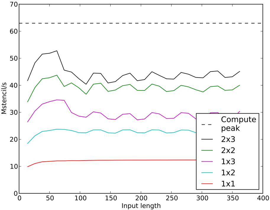
The image is a line graph comparing the performance of different computational configurations (e.g., 2x3, 2x2, 1x3, etc.) in terms of "Mstencil/s" (measured on the y-axis) against "Input length" (x-axis). A dashed horizontal line labeled "Compute peak" at ~60 Mstencil/s serves as a reference. The graph includes five data series with distinct colors and labels, showing varying performance trends across input lengths.
---
### Components/Axes
- **X-axis (Input length)**: Ranges from 0 to 400, with increments of 50. Labeled "Input length."
- **Y-axis (Mstencil/s)**: Ranges from 0 to 70, with increments of 10. Labeled "Mstencil/s."
- **Legend**: Located in the bottom-right corner, with the following mappings:
- **Black dashed line**: "Compute peak" (~60 Mstencil/s).
- **Black solid line**: "2x3" (highest performance).
- **Green solid line**: "2x2" (moderate performance).
- **Purple solid line**: "1x3" (lower performance).
- **Cyan solid line**: "1x2" (lower performance).
- **Red solid line**: "1x1" (lowest performance).
---
### Detailed Analysis
1. **Black solid line (2x3)**:
- Starts at ~42 Mstencil/s at input length 0.
- Peaks at ~52 Mstencil/s around input length 50.
- Fluctuates between ~40–50 Mstencil/s for input lengths 100–400.
- **Trend**: Highest performance, with a sharp initial rise and gradual stabilization.
2. **Green solid line (2x2)**:
- Starts at ~34 Mstencil/s at input length 0.
- Peaks at ~42 Mstencil/s around input length 50.
- Stabilizes between ~38–40 Mstencil/s for input lengths 100–400.
- **Trend**: Moderate performance, with a peak followed by steady values.
3. **Purple solid line (1x3)**:
- Starts at ~28 Mstencil/s at input length 0.
- Peaks at ~34 Mstencil/s around input length 50.
- Fluctuates between ~28–30 Mstencil/s for input lengths 100–400.
- **Trend**: Lower performance, with a peak and gradual decline.
4. **Cyan solid line (1x2)**:
- Starts at ~19 Mstencil/s at input length 0.
- Peaks at ~23 Mstencil/s around input length 50.
- Stabilizes between ~22–23 Mstencil/s for input lengths 100–400.
- **Trend**: Lower performance, with a peak and steady values.
5. **Red solid line (1x1)**:
- Remains flat at ~10 Mstencil/s across all input lengths.
- **Trend**: Constant, lowest performance.
6. **Dashed line (Compute peak)**:
- Horizontal line at ~60 Mstencil/s, above all data series.
- **Trend**: Theoretical maximum, not achieved by any configuration.
---
### Key Observations
- The **2x3 configuration** consistently outperforms others, with the highest Mstencil/s values.
- The **1x1 configuration** is the baseline, showing no improvement with input length.
- All configurations except the 1x1 show a peak around input length 50, followed by stabilization.
- The **Compute peak** (~60 Mstencil/s) is unattainable by any configuration, suggesting a theoretical limit.
---
### Interpretation
The data demonstrates that larger computational configurations (e.g., 2x3) achieve higher performance, but with variability. The 1x1 configuration serves as a baseline, while the Compute peak represents an idealized target. The fluctuations in performance (e.g., 2x3's peaks and troughs) may indicate sensitivity to input length or resource allocation. The absence of any configuration reaching the Compute peak suggests potential bottlenecks or inefficiencies in the system. This graph highlights the trade-off between configuration complexity and performance, with diminishing returns as input length increases.