## Line Graphs: Impulse Response Plots ### Overview The image contains two line graphs, one above the other, displaying impulse response data. Both graphs share the same x-axis (Time in milliseconds) and y-axis (Level). Each graph contains two data series, one in gray and one in black, representing different impulse responses. The initial impulse is significantly larger than subsequent reflections. ### Components/Axes * **X-axis:** Time [ms], ranging from 0 to 40 ms, with gridlines at intervals of 10 ms. * **Y-axis:** Level, ranging from -1.0 to 1.0, with gridlines at intervals of 0.5. * **Data Series:** Each graph contains two data series: one in gray and one in black. There is no explicit legend, but the gray line appears to represent the initial impulse, while the black line represents the subsequent response. ### Detailed Analysis **Top Graph:** * **Gray Line:** The gray line shows a sharp, large initial peak at approximately 0 ms, reaching a level of approximately 0.9. It then rapidly decays to near zero within the first few milliseconds. * **Black Line:** The black line starts near zero and shows several smaller peaks and fluctuations after the initial impulse. These peaks occur between approximately 5 ms and 40 ms, with amplitudes generally below 0.2. The black line appears to be slightly above zero for the entire duration. **Bottom Graph:** * **Gray Line:** Similar to the top graph, the gray line shows a sharp, large initial peak at approximately 0 ms, reaching a level of approximately 0.3. It then rapidly decays to near zero within the first few milliseconds. * **Black Line:** The black line starts near zero and shows several smaller peaks and fluctuations after the initial impulse. These peaks occur between approximately 5 ms and 40 ms, with amplitudes generally below 0.2. The black line appears to be slightly above zero for the entire duration. ### Key Observations * Both graphs show a strong initial impulse followed by a series of smaller reflections or reverberations. * The initial impulse is significantly larger in the top graph (approximately 0.9) compared to the bottom graph (approximately 0.3). * The subsequent reflections (black line) appear to have similar characteristics in both graphs, with peaks generally below 0.2. * The time scale is relatively short (40 ms), suggesting that these are measurements of short-term impulse responses. ### Interpretation The graphs likely represent the impulse response of a system or environment. The initial impulse (gray line) indicates the direct sound or signal, while the subsequent reflections (black line) represent the reverberation or echoes. The difference in the initial impulse amplitude between the top and bottom graphs suggests that the measurements were taken under different conditions, such as different source levels or distances. The similarity in the subsequent reflections suggests that the reverberation characteristics of the environment are relatively consistent between the two measurements. The data suggests that the environment has a short reverberation time, as the reflections decay relatively quickly.

\n ## Chart: Signal Level vs. Time ### Overview The image presents two identical line charts displaying signal level as a function of time. Both charts show a rapid initial drop in signal level followed by a stabilization around zero, with some minor fluctuations. The charts appear to represent the same data, potentially showing replicates or different conditions. ### Components/Axes * **X-axis:** Time [ms], ranging from 0 to 40 milliseconds. The axis is marked with increments of 10 ms. * **Y-axis:** Level, ranging from -1.0 to 1.0. The axis is marked with increments of 0.5. * **Data Series:** A single black line is present in each chart, representing the signal level over time. * **Gridlines:** A grid is overlaid on both charts, aiding in the reading of values. ### Detailed Analysis Both charts exhibit similar behavior. **Chart 1:** * The signal level starts at approximately 0.2 at time 0 ms. * There is a rapid decrease in signal level, reaching a minimum of approximately -0.75 at around 1.5 ms. * Following the initial drop, the signal level oscillates around 0, with fluctuations between approximately -0.2 and 0.2. * From approximately 5 ms to 40 ms, the signal level remains relatively stable, fluctuating within a narrow range around 0. **Chart 2:** * The signal level starts at approximately 0.15 at time 0 ms. * There is a rapid decrease in signal level, reaching a minimum of approximately -0.7 at around 1.5 ms. * Following the initial drop, the signal level oscillates around 0, with fluctuations between approximately -0.2 and 0.2. * From approximately 5 ms to 40 ms, the signal level remains relatively stable, fluctuating within a narrow range around 0. ### Key Observations * Both charts show a very similar initial drop in signal level. * The signal stabilizes around zero after the initial transient. * The fluctuations after the initial drop are relatively small in amplitude. * There is a slight difference in the initial signal level between the two charts. ### Interpretation The charts likely represent a signal response to a step input or a similar triggering event. The initial drop suggests a rapid change in signal state, followed by a settling period where the signal fluctuates around a baseline level of zero. The similarity between the two charts suggests the system is behaving consistently. The slight difference in initial signal level could be due to minor variations in experimental conditions or measurement noise. The data suggests a fast response time (less than 5 ms) and a stable baseline after the initial transient. The charts do not provide information about the nature of the signal or the system generating it, only its temporal behavior.

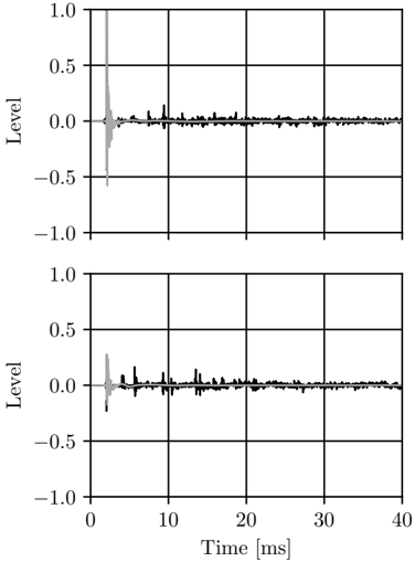
## Line Graphs: Signal Level Over Time ### Overview The image contains two vertically stacked line graphs depicting signal level variations over time. Both graphs share identical axes but represent distinct data series. The top graph shows a pronounced initial spike followed by stabilization, while the bottom graph exhibits a smaller initial spike with persistent low-amplitude fluctuations. ### Components/Axes - **Y-Axis (Level):** - Range: -1.0 to 1.0 - Markers: -1.0, -0.5, 0.0, 0.5, 1.0 - Units: Dimensionless (unitless "Level" metric) - **X-Axis (Time):** - Range: 0 to 40 ms - Markers: 0, 10, 20, 30, 40 ms - Units: Milliseconds - **Graph Structure:** - Two independent line plots (no shared legend or color coding) - Top graph: Sharp vertical spike at 0 ms - Bottom graph: Smaller initial spike with sustained oscillations ### Detailed Analysis 1. **Top Graph (Upper Plot):** - **Initial Spike:** - Occurs at 0 ms - Peaks at approximately 1.0 level - Duration: <1 ms (exact width indeterminate due to resolution) - **Post-Spike Behavior:** - Rapid decay to -0.5 level - Stabilizes near 0.0 level with minor noise (<0.1 level fluctuations) - **Key Data Points:** - (0 ms, 1.0) - (1 ms, -0.5) - (40 ms, ~0.0) 2. **Bottom Graph (Lower Plot):** - **Initial Spike:** - Occurs at 0 ms - Peaks at approximately 0.2 level - Duration: ~2 ms - **Post-Spike Behavior:** - Sustained oscillations between -0.5 and 0.5 - Amplitude: ~0.1-0.2 level - Frequency: ~5-10 Hz (estimated from 40 ms span) - **Key Data Points:** - (0 ms, 0.2) - (2 ms, -0.3) - (40 ms, ~0.1) ### Key Observations 1. Both graphs exhibit transient spikes at t=0 ms, suggesting a shared triggering event. 2. The top graph's spike is 5× more intense than the bottom graph's. 3. Post-spike behavior differs significantly: - Top graph stabilizes - Bottom graph maintains persistent oscillations 4. No correlation between the two data series after t=2 ms. ### Interpretation The data suggests two distinct signal responses to an initial stimulus: 1. **Top Graph:** Represents a high-amplitude, short-duration impulse response with rapid damping. This could indicate a system with strong initial reactivity but fast stabilization (e.g., mechanical shock absorption). 2. **Bottom Graph:** Shows a lower-amplitude, longer-duration oscillatory response. This might represent a resonant system or ongoing feedback mechanism (e.g., electrical circuit with LC oscillations). 3. The absence of shared color coding or legend prevents direct correlation between the two signals, though their temporal alignment at t=0 ms implies a common cause. 4. The persistent noise in both graphs after the initial spike suggests measurement artifacts or environmental interference. No textual content, legends, or additional context is present in the image beyond the axis labels. The graphs appear to be standalone technical measurements without explanatory annotations.