## Line Chart: Throughput vs. Matrix Dimension (m)
### Overview
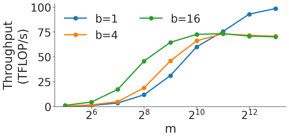
This image displays a line chart illustrating the relationship between computational throughput (measured in TFLOP/s) and a parameter 'm' (likely representing matrix dimension or problem size). The chart compares performance across three different batch sizes ('b'), denoted as $b=1$, $b=4$, and $b=16$. The x-axis is logarithmic, representing powers of 2.
### Components/Axes
* **Y-Axis:** Labeled "Throughput (TFLOP/s)". The scale is linear, ranging from 0 to 100.
* **X-Axis:** Labeled "m". The scale is logarithmic, with major tick marks at $2^6$, $2^8$, $2^{10}$, and $2^{12}$. Data points are plotted at intervals of $2^6, 2^7, 2^8, 2^9, 2^{10}, 2^{11}, 2^{12}, 2^{13}$.
* **Legend:** Located in the top-left quadrant.
* **Blue line:** $b=1$
* **Orange line:** $b=4$
* **Green line:** $b=16$
### Detailed Analysis
The chart plots three distinct series. Below are the approximate values for each data point based on visual estimation:
| X-axis ($m$) | Blue ($b=1$) | Orange ($b=4$) | Green ($b=16$) |
| :--- | :--- | :--- | :--- |
| $2^6$ | ~1 TFLOP/s | ~1 TFLOP/s | ~2 TFLOP/s |
| $2^7$ | ~2 TFLOP/s | ~5 TFLOP/s | ~6 TFLOP/s |
| $2^8$ | ~12 TFLOP/s | ~20 TFLOP/s | ~45 TFLOP/s |
| $2^9$ | ~32 TFLOP/s | ~45 TFLOP/s | ~65 TFLOP/s |
| $2^{10}$ | ~60 TFLOP/s | ~65 TFLOP/s | ~72 TFLOP/s |
| $2^{11}$ | ~75 TFLOP/s | ~75 TFLOP/s | ~73 TFLOP/s |
| $2^{12}$ | ~95 TFLOP/s | ~72 TFLOP/s | ~71 TFLOP/s |
| $2^{13}$ | ~100 TFLOP/s | ~71 TFLOP/s | ~70 TFLOP/s |
**Trend Verification:**
* **Blue ($b=1$):** Starts with the lowest throughput. It exhibits a slow growth initially, followed by a steep, near-linear increase starting around $2^8$, eventually surpassing the other two series at $2^{11}$ and continuing to climb toward 100 TFLOP/s.
* **Orange ($b=4$):** Follows a trajectory similar to the blue line but shifted to the left (earlier performance gains). It plateaus around $2^{11}$ and experiences a slight decline thereafter.
* **Green ($b=16$):** Shows the highest initial throughput at small 'm' values. It rises sharply and plateaus the earliest (around $2^{10}$), after which it remains relatively flat with a slight downward trend.
### Key Observations
* **Crossover Point:** There is a clear crossover at approximately $m = 2^{11}$ (2048). Below this value, higher batch sizes ($b=16$) provide superior throughput. Above this value, the smallest batch size ($b=1$) provides superior throughput.
* **Saturation:** The $b=16$ and $b=4$ configurations appear to hit a performance ceiling (saturation point) around 70-75 TFLOP/s.
* **Scalability:** The $b=1$ configuration demonstrates better scalability for larger 'm' values, as it does not plateau within the visible range of the chart, unlike the $b=4$ and $b=16$ configurations.
### Interpretation
This data is characteristic of a hardware performance benchmark, likely for a GPU or accelerator performing matrix multiplication.
* **Efficiency vs. Overhead:** The higher throughput of $b=16$ at smaller 'm' values suggests that larger batch sizes are more efficient at hiding latency or overhead when the workload is small.
* **Resource Utilization:** The plateauing of $b=4$ and $b=16$ suggests that these configurations hit a hardware bottleneck (likely memory bandwidth or compute unit saturation) earlier than $b=1$.
* **Optimal Configuration:** The choice of 'b' depends heavily on the problem size 'm'. If the workload involves small matrices ($m < 2^{11}$), $b=16$ is optimal. If the workload involves large matrices ($m > 2^{11}$), $b=1$ is significantly more performant. The data suggests that $b=1$ is better optimized for large-scale compute tasks, whereas $b=16$ is better for smaller, latency-sensitive tasks.