## Line Chart: Phase Transition Over Time ### Overview The image is a line chart depicting phase transitions over time. Several lines of different colors show how a variable, phi (φ), changes from an initial value of approximately 0.5 to either 0 or 1 over a time period from 0 to 2. The chart includes the label "DIM" in the bottom-right corner. ### Components/Axes * **X-axis:** * Label: "Time" * Scale: 0 to 2, with markers at 0, 1, and 2. * **Y-axis:** * Label: "φ (π)" * Scale: 0.0 to 1.0, with markers at 0.0, 0.5, and 1.0. * **Data Series:** There are approximately 9 distinct colored lines, each representing a different condition or parameter setting. The colors include dark blue, green, pink, blue, olive, orange, red, teal, and purple. There is no explicit legend. * **Text Label:** "DIM" in the bottom-right corner, colored red. ### Detailed Analysis * **General Trend:** The lines start at φ = 0.5. Some lines transition downwards to φ = 0, while others transition upwards to φ = 1. The transitions occur within the time frame of approximately 0.2 to 1.0. * **Dark Blue Line:** This line starts at φ = 0.5 and decreases to φ = 0. The transition begins around Time = 0.2 and stabilizes at φ = 0 around Time = 0.8. * **Green Line:** This line starts at φ = 0.5 and decreases to φ = 0. The transition begins around Time = 0.3 and stabilizes at φ = 0 around Time = 0.9. * **Pink Line:** This line starts at φ = 0.5 and decreases to φ = 0. The transition begins around Time = 0.35 and stabilizes at φ = 0 around Time = 0.9. * **Blue Line:** This line starts at φ = 0.5 and decreases to φ = 0. The transition begins around Time = 0.4 and stabilizes at φ = 0 around Time = 0.95. * **Olive Line:** This line starts at φ = 0.5 and decreases to φ = 0. The transition begins around Time = 0.45 and stabilizes at φ = 0 around Time = 1.0. * **Orange Line:** This line starts at φ = 0.5 and increases to φ = 1. The transition begins around Time = 0.4 and stabilizes at φ = 1 around Time = 0.9. * **Red Line:** This line starts at φ = 0.5 and increases to φ = 1. The transition begins around Time = 0.35 and stabilizes at φ = 1 around Time = 0.8. * **Teal Line:** This line starts at φ = 0.5 and increases to φ = 1. The transition begins around Time = 0.3 and stabilizes at φ = 1 around Time = 0.75. * **Purple Line:** This line starts at φ = 0.5 and increases to φ = 1. The transition begins around Time = 0.45 and stabilizes at φ = 1 around Time = 0.9. ### Key Observations * The lines exhibit a clear bifurcation, with some transitioning to 0 and others to 1. * The transitions occur within a relatively narrow time window. * The "DIM" label is present but its significance is not immediately clear without additional context. ### Interpretation The chart likely represents a system undergoing a phase transition, where the initial state (φ = 0.5) is unstable, and the system evolves towards one of two stable states (φ = 0 or φ = 1). The different colored lines could represent different initial conditions or parameter settings that influence the direction and speed of the transition. The "DIM" label might refer to the specific system or model being studied. The data suggests that the system is sensitive to initial conditions or parameter variations, leading to the observed bifurcation.

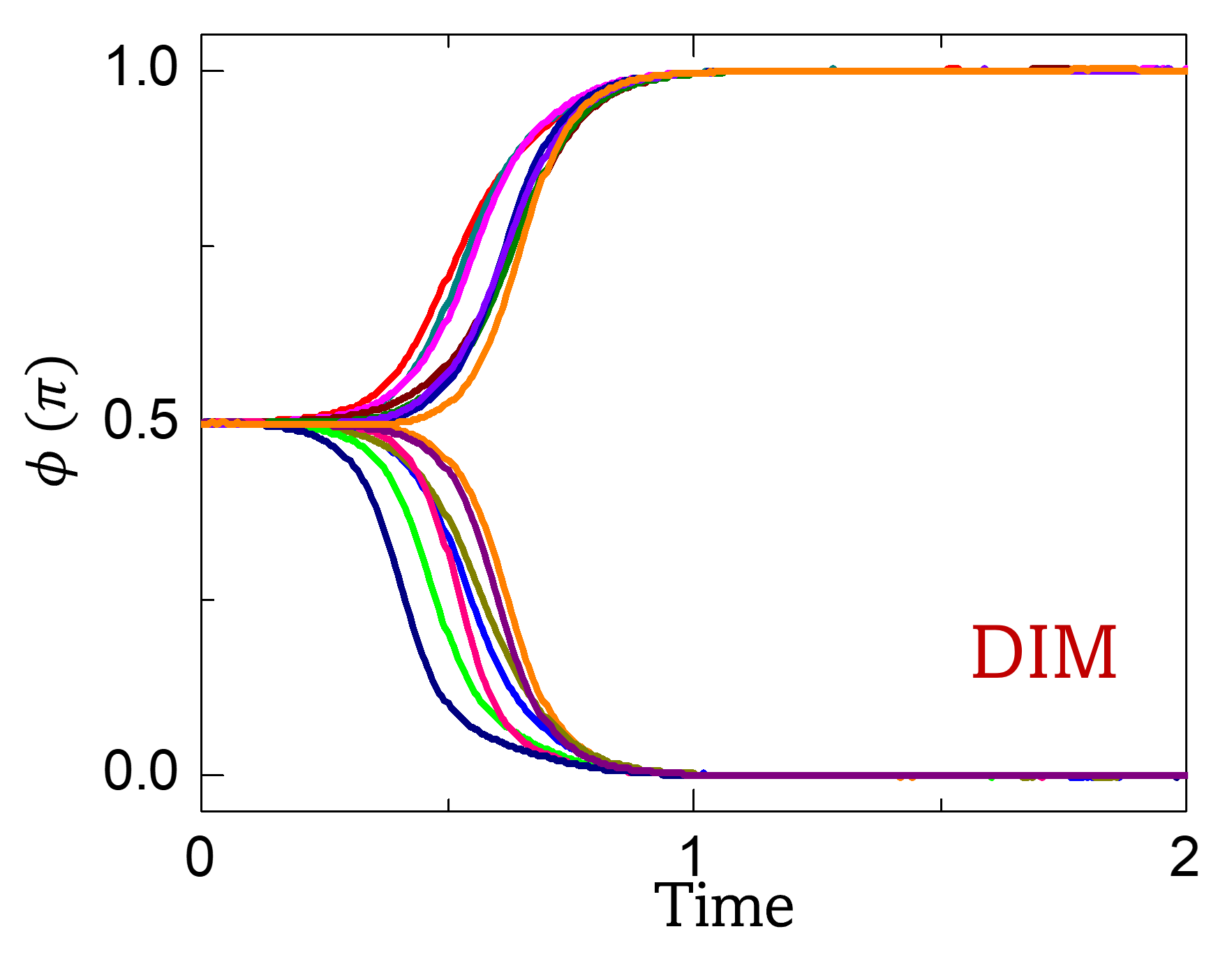
## Line Chart: Bifurcation of $\phi (\pi)$ over Time ### Overview The image displays a line chart illustrating the temporal evolution of a variable, denoted as $\phi (\pi)$, starting from a neutral state of 0.5. The chart demonstrates a bifurcation process where multiple trajectories, initially clustered at 0.5, diverge over time to settle into one of two stable states: 0.0 or 1.0. The chart includes the annotation "DIM" in the lower-right quadrant. ### Components/Axes * **Y-Axis**: Labeled "$\phi (\pi)$". The scale ranges from 0.0 to 1.0. Major tick marks are present at 0.0, 0.5, and 1.0. * **X-Axis**: Labeled "Time". The scale ranges from 0 to 2. Major tick marks are present at 0, 1, and 2. * **Data Series**: Multiple colored lines (magenta, light blue, green, dark blue, orange, brown) representing different simulation runs or parameter variations. * **Annotation**: The text "DIM" is written in red, positioned in the lower-right area of the chart (approximately at x=1.5, y=0.25). ### Detailed Analysis * **Initial State (t = 0 to ~0.3)**: All data series originate at the coordinate (0, 0.5). The lines remain tightly clustered, showing no significant deviation from the 0.5 value during this initial phase. * **Divergence Phase (~0.3 to ~0.8)**: Starting at approximately t=0.3, the lines begin to diverge. * **Upper Branch**: A subset of lines (magenta, light blue, orange, brown) curves upward, increasing monotonically toward the value of 1.0. * **Lower Branch**: A subset of lines (dark blue, green, brown, orange) curves downward, decreasing monotonically toward the value of 0.0. * **Steady State (~0.8 to 2.0)**: By t=0.8, all lines have reached their respective steady states. The lines remain flat at either 0.0 or 1.0 for the remainder of the time axis (up to t=2.0). * **Symmetry**: The bifurcation appears largely symmetric around the horizontal line $\phi = 0.5$. ### Key Observations * **Bistability**: The system exhibits clear bistable behavior. The state $\phi = 0.5$ acts as an unstable equilibrium point, while 0.0 and 1.0 act as stable attractors. * **Transition Speed**: The transition from the unstable equilibrium to the stable attractors is rapid, occurring over a time interval of approximately 0.5 units. * **Annotation**: The red "DIM" label is isolated from the axes and data, suggesting it is a label for the specific dataset or model configuration being plotted, rather than a variable on the axes. ### Interpretation The data suggests a phase transition or a bifurcation event in a dynamical system. The system is initially in a state of unstable equilibrium ($\phi = 0.5$). As time progresses, the system is forced to "choose" between two stable outcomes (0.0 or 1.0). The "DIM" label likely stands for "Dimensionality" or refers to a specific parameter set (e.g., "Dimension 1" or "Dimensionality reduction"). In computational or physical modeling, this type of plot is characteristic of systems undergoing symmetry breaking, where small variations in initial conditions or parameters lead to divergent macroscopic outcomes. The fact that all lines converge to exactly 0.0 or 1.0 indicates that the system is highly constrained or "saturated" once the transition is complete.

## Line Graph: φ(π) vs. Time with Divergent Paths ### Overview The image depicts a line graph showing the behavior of a function φ(π) over time. Multiple colored lines originate from a common point at (Time = 0.5, φ(π) = 0.5) and diverge into distinct paths. The graph includes a legend labeled "DIM" in red, though the colors of the lines are not explicitly explained in the legend. The x-axis (Time) ranges from 0 to 2, and the y-axis (φ(π)) ranges from 0.0 to 1.0. --- ### Components/Axes - **X-axis (Time)**: Labeled "Time" with values from 0 to 2. - **Y-axis (φ(π))**: Labeled "φ(π)" with values from 0.0 to 1.0. - **Legend**: Located in the bottom-right corner, labeled "DIM" in red. No explicit color-to-label mapping is provided for the lines. - **Lines**: Multiple colored lines (red, blue, green, purple, orange, etc.) originate from the point (0.5, 0.5) and diverge into different trajectories. --- ### Detailed Analysis 1. **Initial Convergence**: All lines start at the same point (Time = 0.5, φ(π) = 0.5), suggesting a shared initial condition or critical threshold. 2. **Divergence Paths**: - **Red Line**: Ascends sharply to φ(π) = 1.0 by Time = 1.0, then remains flat. - **Blue Line**: Descends sharply to φ(π) = 0.0 by Time = 1.0, then remains flat. - **Green Line**: Rises to φ(π) ≈ 0.8 by Time = 1.0, then plateaus. - **Purple Line**: Drops to φ(π) ≈ 0.2 by Time = 1.0, then plateaus. - **Orange Line**: Remains flat at φ(π) = 0.5 throughout the entire time range. 3. **Unlabeled Colors**: Additional lines (e.g., teal, brown, pink) exhibit intermediate trends, but their exact paths are not clearly distinguishable due to overlapping or low contrast. --- ### Key Observations - **Critical Point at Time = 0.5**: All lines originate from the same point, indicating a shared initial state or bifurcation event. - **Divergence Patterns**: Lines exhibit distinct behaviors (ascending, descending, flat) after Time = 0.5, suggesting varying responses to an underlying parameter or condition. - **Unlabeled Legend**: The legend "DIM" in red does not clarify the meaning of the colored lines, leaving their interpretation ambiguous. - **Flat Lines**: The orange line (and possibly others) remains constant, implying a steady-state or equilibrium condition. --- ### Interpretation The graph likely represents a dynamical system or model where φ(π) evolves over time under different scenarios labeled as "DIM." The convergence at Time = 0.5 suggests a critical transition or bifurcation point, after which the system branches into multiple outcomes. The flat lines (e.g., orange) may represent stable equilibria, while the ascending/descending lines indicate dynamic changes. The absence of a clear legend for the colored lines limits the ability to assign specific meanings to each path. However, the overall structure implies that "DIM" could be a parameter or model influencing the system's behavior, with different trajectories reflecting varying conditions or inputs.