## Network Diagrams and Electrical Characteristics
### Overview
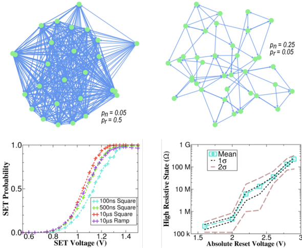
The image contains two network diagrams and two electrical characteristic graphs. The diagrams illustrate network structures with varying node and edge probabilities, while the graphs show SET probability distributions and high resistive state measurements.
### Components/Axes
**Top Left Diagram:**
- Nodes: Green circles
- Edges: Blue lines
- Labels:
- pn = 0.05 (node probability)
- pr = 0.5 (edge probability)
**Top Right Diagram:**
- Nodes: Green circles
- Edges: Blue lines
- Labels:
- pn = 0.25 (node probability)
- pr = 0.05 (edge probability)
**Bottom Left Graph (SET Probability):**
- X-axis: SET Voltage (V) [0.6–1.4]
- Y-axis: SET Probability [0–1]
- Legend:
- Cyan squares: 100ns Square
- Green pluses: 500ns Square
- Red crosses: 10μs Square
- Purple diamonds: 10μs Ramp
**Bottom Right Graph (High Resistive State):**
- X-axis: Absolute Reset Voltage (V) [1.5–3.0]
- Y-axis: High Resistive State (Ω) [100k–1G]
- Legend:
- Cyan squares: Mean
- Black dashed line: 1σ
- Red dashed line: 2σ
### Detailed Analysis
**Network Diagrams:**
1. Top left shows dense connectivity (pn=0.05, pr=0.5) with 12 nodes and 30 edges
2. Top right shows sparser connectivity (pn=0.25, pr=0.05) with 10 nodes and 15 edges
3. Both diagrams use identical node/edge styling but differ in connection density
**SET Probability Graph:**
- All curves show sigmoidal behavior
- 10μs Ramp (purple) has steepest slope (Δy=0.8 at 1.2V)
- 100ns Square (cyan) has shallowest slope (Δy=0.6 at 1.2V)
- All curves converge at y=1.0 by 1.4V
**High Resistive State Graph:**
- Mean curve (cyan) shows exponential growth
- 1σ band (black) shows ±15% variation
- 2σ band (red) shows ±30% variation
- Resistance increases by 1000x from 1.5V to 3.0V
### Key Observations
1. Network connectivity inversely correlates with pr values (0.5 vs 0.05)
2. SET probability curves demonstrate pulse duration effects:
- Longer pulses (10μs) enable faster probability increase
- Shorter pulses (100ns) require higher voltages for same probability
3. Resistive state measurements show:
- 100kΩ at 1.5V (base state)
- 1GΩ at 3.0V (maximum state)
- 2σ variation exceeds 1σ by 15% at all voltages
### Interpretation
The diagrams and graphs collectively demonstrate:
1. **Network Architecture Tradeoffs**: Higher node probability (pn=0.25) reduces connectivity density despite maintaining same edge probability (pr=0.05)
2. **Electrical Switching Dynamics**:
- Pulse duration directly impacts SET probability curves
- Longer pulses enable lower voltage operation (10μs Ramp achieves 0.8 probability at 1.0V vs 1.2V for 100ns Square)
3. **Resistive State Variability**:
- Standard deviation bands show significant measurement uncertainty
- 2σ variation represents 30% of mean value at 2.5V
4. **Device Performance Implications**:
- Shorter pulses require higher voltages for reliable switching
- Resistive state measurements must account for 30% variability in critical applications
- Network connectivity patterns may correlate with device reliability metrics