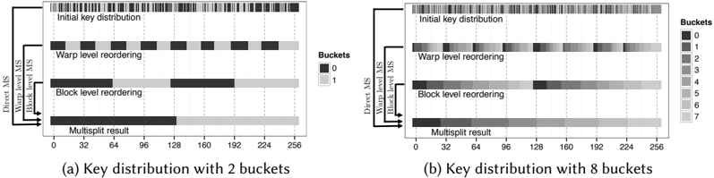
## Key Distribution Diagram: 2 Buckets vs. 8 Buckets ### Overview The image presents two diagrams illustrating key distribution during a multi-split process. Diagram (a) shows the distribution with 2 buckets, while diagram (b) shows the distribution with 8 buckets. Each diagram depicts the initial key distribution, the reordering at warp and block levels, and the final multi-split result. The diagrams use grayscale to represent different buckets. ### Components/Axes **Diagram (a): Key distribution with 2 buckets** * **Title:** (a) Key distribution with 2 buckets * **X-axis:** Numerical scale from 0 to 256, with markers at 0, 32, 64, 96, 128, 160, 192, 224, and 256. * **Y-axis:** Implicitly represents the stages of key distribution. * **Legend (Buckets):** Located on the right side. * Dark gray represents bucket 0. * Light gray represents bucket 1. * **Stages:** * Initial key distribution: Shows a sparse distribution of keys. * Warp level reordering: Shows keys grouped into blocks. * Block level reordering: Shows a more consolidated distribution. * Multisplit result: Shows a relatively even distribution of keys across the range. * **Arrows:** Three arrows labeled "Direct MS", "Warp level MS", and "Block level MS" point from left to right, indicating the flow of the multi-split process. **Diagram (b): Key distribution with 8 buckets** * **Title:** (b) Key distribution with 8 buckets * **X-axis:** Numerical scale from 0 to 256, with markers at 0, 32, 64, 96, 128, 160, 192, 224, and 256. * **Y-axis:** Implicitly represents the stages of key distribution. * **Legend (Buckets):** Located on the right side. * Darkest gray represents bucket 0. * Progressively lighter shades of gray represent buckets 1 through 7. * **Stages:** * Initial key distribution: Shows a sparse distribution of keys. * Warp level reordering: Shows keys grouped into blocks. * Block level reordering: Shows a more consolidated distribution. * Multisplit result: Shows a relatively even distribution of keys across the range. * **Arrows:** Three arrows labeled "Direct MS", "Warp level MS", and "Block level MS" point from left to right, indicating the flow of the multi-split process. ### Detailed Analysis **Diagram (a): Key distribution with 2 buckets** * **Initial key distribution:** Keys are sparsely distributed, with more keys concentrated in the left half (0-128) than the right half (128-256). * **Warp level reordering:** Keys are grouped into four distinct blocks. The first and third blocks are dark gray (bucket 0), while the second and fourth blocks are light gray (bucket 1). * **Block level reordering:** The distribution is consolidated into two blocks. The left block is approximately 128 units long and is dark gray (bucket 0). The right block is approximately 128 units long and is light gray (bucket 1). * **Multisplit result:** The keys are distributed evenly across the entire range (0-256), with the left half being dark gray (bucket 0) and the right half being light gray (bucket 1). **Diagram (b): Key distribution with 8 buckets** * **Initial key distribution:** Keys are sparsely distributed, with a higher concentration in the left half (0-128) than the right half (128-256). * **Warp level reordering:** Keys are grouped into several blocks, each representing a different bucket (0-7) in grayscale. * **Block level reordering:** The distribution is consolidated into several blocks, each representing a different bucket (0-7) in grayscale. * **Multisplit result:** The keys are distributed evenly across the entire range (0-256), with each section representing a different bucket (0-7) in grayscale. ### Key Observations * Both diagrams show a progression from a sparse initial key distribution to a more even distribution after the multi-split process. * The warp and block level reordering stages show intermediate steps in consolidating and grouping keys. * The number of buckets significantly impacts the granularity of the final key distribution. With 2 buckets, the final distribution is divided into two halves, while with 8 buckets, the final distribution is divided into eight sections. ### Interpretation The diagrams illustrate the process of key distribution in a multi-split operation. The initial key distribution is often uneven, which can lead to performance bottlenecks. The warp and block level reordering stages aim to consolidate and group keys to improve efficiency. The multi-split result shows the final distribution of keys across the buckets. The comparison between 2 buckets and 8 buckets highlights the trade-off between granularity and overhead. With more buckets, the distribution can be more even, but the overhead of managing more buckets increases. The choice of the number of buckets depends on the specific application and the characteristics of the data.

\n ## Heatmaps: Key Distribution with Varying Buckets ### Overview The image presents two heatmaps, labeled (a) and (b), illustrating the distribution of keys across different processing stages. Both heatmaps visualize the effect of various reordering techniques (Direct MS, Warp Level MS, Block Level MS, and Multisplit) on an initial key distribution. Heatmap (a) uses 2 buckets, while heatmap (b) uses 8 buckets for representing the key distribution. The intensity of the color represents the density of keys within each bucket at each processing stage. ### Components/Axes Both heatmaps share the following components: * **Y-axis:** Represents the processing stages: "Initial key distribution", "Warp level reordering", "Block level reordering", and "Multisplit result". The order is from top to bottom. * **X-axis:** Represents the key values, ranging from 0 to 256. The scale is linear. * **Color Scale/Legend:** * **(a):** Two colors: Black (representing bucket 0) and White (representing bucket 1). * **(b):** Eight colors, ranging from Black to White, representing buckets 0 through 7. * **Labels:** Each heatmap is labeled with "(a) Key distribution with 2 buckets" and "(b) Key distribution with 8 buckets" respectively. ### Detailed Analysis or Content Details **Heatmap (a) - 2 Buckets:** * **Initial key distribution:** The keys are heavily concentrated towards the lower end of the range (0-64), primarily in bucket 0 (black). There's a small presence of bucket 1 (white) towards the higher end (around 224-256). * **Warp level reordering:** The distribution becomes more spread out, with bucket 0 (black) still dominant in the lower range (0-96) and bucket 1 (white) appearing more frequently in the upper range (96-256). * **Block level reordering:** The distribution is further spread out. Bucket 0 (black) is present from 0-128, and bucket 1 (white) is present from 128-256. * **Multisplit result:** The distribution is relatively uniform, with a mix of bucket 0 (black) and bucket 1 (white) across the entire range, though still slightly more concentrated towards the lower end. **Heatmap (b) - 8 Buckets:** * **Initial key distribution:** The keys are concentrated towards the lower end (0-64), with a gradient of buckets from 0 (black) to 2 (grey). Higher buckets (3-7) are sparsely present towards the upper end (224-256). * **Warp level reordering:** The distribution becomes more spread out. Buckets 0-3 (black to light grey) are present in the lower range (0-128), and buckets 3-7 are present in the upper range (128-256). * **Block level reordering:** The distribution is even more spread out. Buckets 0-5 are present in the lower range (0-192), and buckets 3-7 are present in the upper range (192-256). * **Multisplit result:** The distribution is the most uniform, with all buckets (0-7) present across the entire range, though there's a slight gradient, with lower buckets being more prevalent in the lower range and higher buckets in the upper range. ### Key Observations * As the processing stages progress, the key distribution becomes more uniform in both heatmaps. * Increasing the number of buckets (from 2 to 8) reveals a more granular distribution of keys. * The "Multisplit result" consistently demonstrates the most uniform distribution across all buckets. * The initial key distribution is heavily skewed towards lower key values. ### Interpretation These heatmaps demonstrate the effectiveness of different reordering techniques in distributing keys more evenly. The initial key distribution is highly non-uniform, which can lead to performance bottlenecks in parallel processing. The reordering techniques, particularly "Block level reordering" and "Multisplit result", aim to mitigate this issue by spreading the keys across a wider range of buckets. The transition from 2 buckets to 8 buckets provides a more detailed view of the distribution, revealing subtle differences in the effectiveness of each technique. The "Multisplit result" consistently achieves the most uniform distribution, suggesting it is the most effective method for balancing the workload across processing units. The color gradients in heatmap (b) indicate that while the distribution is more uniform, there's still a slight bias towards lower key values, even after the reordering process. This suggests that further optimization might be possible to achieve a perfectly uniform distribution. The heatmaps provide a visual representation of how these techniques impact key distribution, which is crucial for understanding and optimizing parallel processing performance.

## Technical Diagram: Key Distribution and Reordering Process ### Overview The image displays two side-by-side technical diagrams illustrating a parallel computing process for sorting or partitioning data keys. The diagrams compare the process using two different numbers of output buckets (2 and 8). The process involves multiple stages of reordering, moving from an initial random distribution to a final sorted result. ### Components/Axes **Common Elements (Both Diagrams):** * **Vertical Flow:** The process flows from top to bottom through four distinct stages. * **Stage Labels (Left Side):** * Initial key distribution * Warp level reordering * Block level reordering * Multisplit result * **Control Flow Arrows (Left Side):** Arrows indicate the flow of data/control between stages, labeled with technical terms: * Direct MS * Warp MS * Block MS * **Horizontal Axis (Bottom):** Labeled "Key Index," with numerical markers at 0, 32, 64, 96, 128, 160, 192, 224, and 256. This represents the position or index of individual data keys. * **Legend (Right Side):** A legend titled "Buckets" maps colors/shades to bucket numbers. **Diagram-Specific Elements:** * **(a) Left Diagram:** Titled "(a) Key distribution with 2 buckets." Its legend shows two buckets: Bucket 0 (black) and Bucket 1 (light gray). * **(b) Right Diagram:** Titled "(b) Key distribution with 8 buckets." Its legend shows eight buckets, numbered 0 through 7, represented by a gradient from black (0) to light gray (7). ### Detailed Analysis **Diagram (a): Key distribution with 2 buckets** 1. **Initial key distribution:** A horizontal bar shows a seemingly random, high-frequency alternation between black and light gray pixels, indicating keys are randomly assigned to Bucket 0 or 1 across the entire index range (0-256). 2. **Warp level reordering:** The bar shows a pattern of short, alternating black and light gray segments. The reordering has begun to locally group keys of the same bucket within small, contiguous blocks (likely corresponding to GPU "warps"). 3. **Block level reordering:** The bar shows larger, more consolidated blocks of color. A large black segment spans approximately indices 0-128, followed by a large light gray segment from ~128-256. This indicates keys have been successfully partitioned into two major groups at a coarse granularity. 4. **Multisplit result:** The final bar shows a perfect partition: a solid black segment from index 0 to 128, and a solid light gray segment from index 128 to 256. All keys for Bucket 0 are contiguous at the start, and all keys for Bucket 1 are contiguous at the end. **Diagram (b): Key distribution with 8 buckets** 1. **Initial key distribution:** A horizontal bar shows a very fine-grained, noisy pattern of eight different shades, indicating keys are randomly assigned to one of eight buckets across all indices. 2. **Warp level reordering:** The bar shows a pattern where the eight shades begin to form small, localized clusters, but the overall distribution is still mixed. 3. **Block level reordering:** The bar shows clearer, larger bands of similar shades. The keys are being grouped into broader ranges corresponding to their bucket values, though the boundaries are not yet perfectly sharp. 4. **Multisplit result:** The final bar shows a perfect, sorted partition. The keys are arranged in eight contiguous, solid-colored bands in order from Bucket 0 (black, leftmost) to Bucket 7 (light gray, rightmost). The boundaries between buckets appear to be at non-uniform indices (e.g., Bucket 0 ends near index 32, Bucket 1 near 64, etc.), indicating the final distribution of keys per bucket is not equal. ### Key Observations * **Progressive Ordering:** Both diagrams demonstrate a clear trend of increasing order from the top (random) to the bottom (fully sorted) stage. * **Hierarchical Reordering:** The process uses a two-level hierarchy ("Warp level" then "Block level") to achieve the final partition, which is a common optimization pattern in parallel computing (e.g., GPU algorithms). * **Bucket Granularity Impact:** The 2-bucket case results in a simple binary split at the midpoint. The 8-bucket case results in a more complex, multi-way partition where the final segment lengths (number of keys per bucket) are unequal, reflecting the initial random distribution. * **Visual Metaphor:** The diagrams effectively use a horizontal bar of colored pixels as a metaphor for an array of data, where color represents a key's bucket assignment and position represents its index in memory. ### Interpretation This diagram illustrates the **Multisplit** operation, a fundamental primitive in parallel computing for partitioning an array of elements into multiple buckets based on their keys. This is a critical step in algorithms like parallel sorting (e.g., sample sort) or in distributed computing for data redistribution. The process shown is a **hierarchical parallel partitioning algorithm**. It first performs local reordering within small thread groups ("warps"), then performs a global reordering across larger thread groups ("blocks"). This two-phase approach minimizes expensive global communication and maximizes local memory coherence, which is essential for performance on architectures like GPUs. The key takeaway is the transformation from entropy (random distribution) to order (sorted buckets). The "Multisplit result" bars provide a visual proof of the algorithm's correctness. The difference between the 2-bucket and 8-bucket results highlights the algorithm's scalability to handle multiple partitions, a necessity for efficient large-scale sorting. The unequal final segment lengths in (b) are not an anomaly but an expected outcome, demonstrating that the algorithm correctly handles arbitrary key distributions.

## Chart/Diagram Type: Key Distribution Visualization with Reordering Stages ### Overview The image contains two side-by-side diagrams comparing key distribution patterns across different reordering stages (Warp level and Block level) for two scenarios: (a) 2 buckets and (b) 8 buckets. Each diagram shows the evolution of key distribution from initial state through reordering processes to a final multisplit result. ### Components/Axes **Left Diagram (2 Buckets):** - **X-axis**: "Buckets" with markers at 0, 32, 64, 96, 128, 160, 192, 224, 256 - **Y-axis**: Processing stages labeled: - Initial key distribution - Warp level reordering - Block level reordering - Multisplit result - **Legend**: - Black = Bucket 0 - Gray = Bucket 1 - **Spatial Layout**: Legend positioned right-aligned, stages stacked vertically from top to bottom **Right Diagram (8 Buckets):** - **X-axis**: Same bucket markers as left diagram - **Y-axis**: Same processing stages - **Legend**: - 8 grayscale shades representing buckets 0-7 - **Spatial Layout**: Identical to left diagram but with more granular legend ### Detailed Analysis **Left Diagram (2 Buckets):** 1. **Initial Distribution**: Alternating black/gray bars (0-1 pattern) 2. **Warp Level Reordering**: - Bars grouped into 4 black/gray pairs - Each pair spans ~32-64 units 3. **Block Level Reordering**: - Two large blocks: - First block: ~64 units (black) - Second block: ~128 units (gray) 4. **Multisplit Result**: Single gray bar spanning entire width (~256 units) **Right Diagram (8 Buckets):** 1. **Initial Distribution**: - 16 alternating gray shades (0-7 pattern) - Each bar ~16 units wide 2. **Warp Level Reordering**: - Bars grouped into 8 clusters - Each cluster spans ~32 units 3. **Block Level Reordering**: - Four large blocks: - First block: ~64 units (buckets 0-3) - Second block: ~128 units (buckets 4-7) 4. **Multisplit Result**: Single dark gray bar spanning entire width ### Key Observations 1. **Bucket Granularity Impact**: - 8-bucket version shows 4x more detailed initial distribution - Warp level reordering in 8-bucket version maintains finer granularity 2. **Reordering Effectiveness**: - Both versions show progressive consolidation through stages - Block level reordering creates larger contiguous blocks 3. **Multisplit Consistency**: - Final result identical in both diagrams (single bar) - Suggests final consolidation is bucket-count agnostic 4. **Block Level Differences**: - 2-bucket version shows more extreme consolidation (2 blocks vs 4 in 8-bucket) ### Interpretation The diagrams demonstrate how key distribution evolves through hierarchical reordering processes. The 8-bucket version maintains finer granularity throughout all stages compared to the 2-bucket version, suggesting that initial bucket count affects intermediate distribution patterns but not the final consolidated result. The block level reordering appears to be the most impactful stage, reducing distribution complexity by ~50% in both cases. The consistent final multisplit result across both scenarios implies that the reordering algorithm effectively normalizes distribution regardless of initial bucket configuration, though the 8-bucket version provides more detailed intermediate insights. This visualization could be used to optimize key distribution strategies by analyzing intermediate reordering stages.