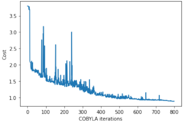
## Line Graph: COBYLA Cost vs. Iterations ### Overview The image depicts a line graph illustrating the relationship between the number of COBYLA iterations and the associated cost. The graph shows a decreasing trend in cost over iterations, with notable fluctuations in the early stages. The y-axis represents "Cost" (ranging from 1.0 to 3.5), and the x-axis represents "COBYLA iterations" (ranging from 0 to 800). A single blue line, labeled "COBYLA" in the legend, tracks the cost metric across iterations. ### Components/Axes - **X-axis (Horizontal)**: Labeled "COBYLA iterations," with a linear scale from 0 to 800 in increments of 100. - **Y-axis (Vertical)**: Labeled "Cost," with a linear scale from 1.0 to 3.5 in increments of 0.5. - **Legend**: Positioned in the top-right corner, indicating that the blue line corresponds to the "COBYLA" data series. - **Line**: A single blue line representing the cost metric across iterations. ### Detailed Analysis - **Initial Spike**: At iteration 0, the cost begins at approximately **3.5**, dropping sharply to ~2.0 by iteration 50. - **Early Fluctuations**: Between iterations 50 and 200, the cost oscillates between ~1.5 and ~2.5, with several sharp spikes (e.g., ~2.8 at iteration 150, ~2.2 at iteration 180). - **Gradual Decline**: From iteration 200 to 500, the cost trends downward, stabilizing around ~1.2 by iteration 400, with minor fluctuations (e.g., ~1.4 at iteration 350). - **Late-Stage Stability**: From iteration 500 to 800, the cost remains relatively flat, hovering between ~1.0 and ~1.1, with occasional small spikes (e.g., ~1.15 at iteration 700). ### Key Observations 1. **Initial Volatility**: The first 200 iterations exhibit significant cost variability, suggesting instability or sensitivity to initial conditions. 2. **Convergence**: After iteration 400, the cost stabilizes, indicating convergence toward an optimal solution. 3. **Spike Patterns**: Spikes occur sporadically (e.g., iterations 150, 180, 350), potentially reflecting local minima or parameter adjustments in the COBYLA algorithm. ### Interpretation The graph demonstrates that the COBYLA algorithm effectively reduces cost over iterations, with a clear downward trend after the initial volatile phase. The stabilization of cost after iteration 400 suggests that the algorithm has reached a near-optimal solution. The early spikes may indicate transient inefficiencies or exploration of suboptimal regions in the search space. The final stable cost (~1.0–1.1) implies successful optimization, though the exact nature of the cost function (e.g., minimization of error, resource allocation) is not specified. The absence of additional data series or parameters limits deeper analysis of algorithmic behavior.