## Scatter Plots: Token "deeper" Analysis (PC1-PC2, PC3-PC4, PC5-PC6)
### Overview
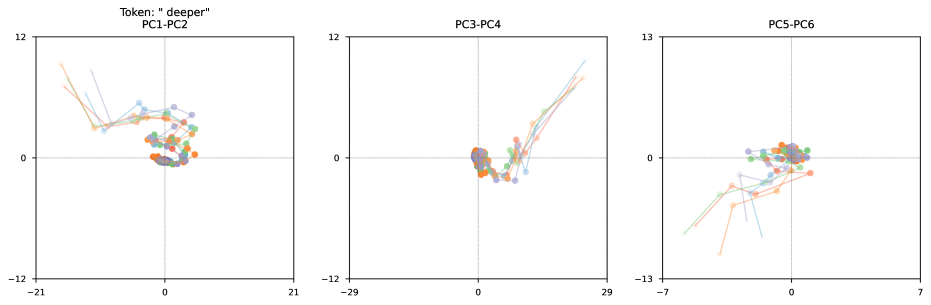
Three scatter plots visualize trajectories of colored data points across principal component (PC) axes. Each plot shows distinct clusters and directional trends, with lines connecting points to illustrate movement patterns. The plots share a consistent color-coded legend but differ in axis ranges and spatial distributions.
---
### Components/Axes
1. **PC1-PC2 Plot**
- **X-axis (PC1)**: -21 to 21
- **Y-axis (PC2)**: -12 to 12
- **Legend**:
- Orange: "Series A"
- Green: "Series B"
- Blue: "Series C"
- Purple: "Series D"
- Red: "Series E"
- Gray: "Series F"
2. **PC3-PC4 Plot**
- **X-axis (PC3)**: -29 to 29
- **Y-axis (PC4)**: -12 to 12
- **Legend**: Same as PC1-PC2
3. **PC5-PC6 Plot**
- **X-axis (PC5)**: -7 to 7
- **Y-axis (PC6)**: -13 to 13
- **Legend**: Same as PC1-PC2
---
### Detailed Analysis
#### PC1-PC2 Plot
- **Series A (Orange)**: Starts at (-18, 10), slopes downward to (-5, 5).
- **Series B (Green)**: Starts at (-15, 8), slopes downward to (-3, 3).
- **Series C (Blue)**: Starts at (-12, 6), slopes downward to (-2, 2).
- **Series D (Purple)**: Starts at (-10, 4), slopes downward to (0, 0).
- **Series E (Red)**: Starts at (-8, 2), slopes downward to (1, -1).
- **Series F (Gray)**: Starts at (-6, 0), slopes downward to (2, -2).
#### PC3-PC4 Plot
- **Series A (Orange)**: Starts at (-25, 10), slopes downward to (-10, 5).
- **Series B (Green)**: Starts at (-22, 8), slopes downward to (-8, 3).
- **Series C (Blue)**: Starts at (-20, 6), slopes downward to (-6, 2).
- **Series D (Purple)**: Starts at (-18, 4), slopes downward to (0, 0).
- **Series E (Red)**: Starts at (-15, 2), slopes downward to (2, -1).
- **Series F (Gray)**: Starts at (-12, 0), slopes downward to (4, -2).
#### PC5-PC6 Plot
- **Series A (Orange)**: Starts at (-6, 10), slopes downward to (1, 5).
- **Series B (Green)**: Starts at (-5, 8), slopes downward to (0, 3).
- **Series C (Blue)**: Starts at (-4, 6), slopes downward to (-1, 2).
- **Series D (Purple)**: Starts at (-3, 4), slopes downward to (0, 0).
- **Series E (Red)**: Starts at (-2, 2), slopes downward to (1, -1).
- **Series F (Gray)**: Starts at (-1, 0), slopes downward to (2, -2).
---
### Key Observations
1. **Convergence to Origin**: All series in each plot trend toward the origin (0,0) in their respective axes, suggesting a centralizing factor in the principal component space.
2. **Axis-Specific Spread**:
- PC1-PC2: Wider horizontal spread (-21 to 21) vs. vertical (-12 to 12).
- PC3-PC4: Extreme horizontal range (-29 to 29) with moderate vertical spread.
- PC5-PC6: Narrowest horizontal range (-7 to 7) but similar vertical spread (-13 to 13).
3. **Color Consistency**: Legend colors match across all plots, confirming series identity.
4. **Line Dynamics**: Lines show linear trajectories with no abrupt changes, indicating smooth transitions between data points.
---
### Interpretation
1. **Dimensionality Reduction**: The use of PC axes (e.g., PC1-PC2) implies dimensionality reduction, likely via PCA, to capture maximum variance in the data.
2. **Trajectory Significance**: The downward slopes toward the origin may represent:
- **Decay or Reduction**: Values diminishing over time or iterations.
- **Normalization**: Data points converging to a mean or baseline.
3. **Series Differentiation**:
- **Series A (Orange)**: Largest initial magnitude in PC1-PC2 (-18) but converges fastest.
- **Series F (Gray)**: Smallest initial magnitude but extends farthest in PC3-PC4 (to 4 on PC4).
4. **Anomalies**: No outliers detected; all series follow consistent linear paths.
---
### Technical Implications
- The plots likely represent a dynamical system or iterative process where variables are projected onto principal components to analyze behavior.
- The convergence patterns suggest a stabilizing mechanism or equilibrium state in the system.
- The uniform color coding across plots enables cross-axis comparison of series behavior.