## Histogram: Bimodal Distribution of Interval Probabilities
### Overview
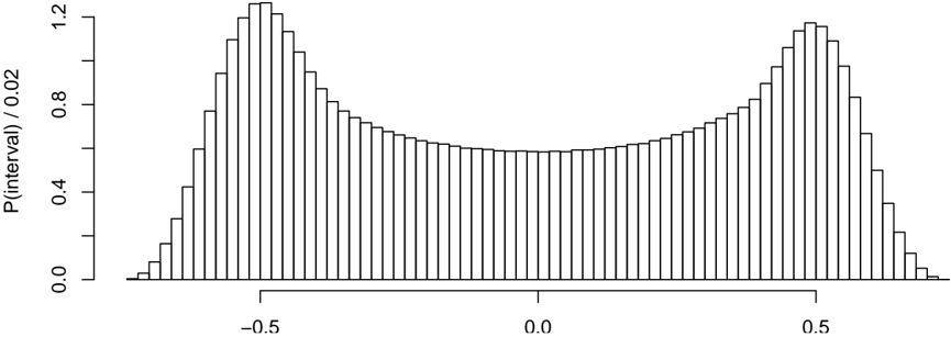
The image displays a histogram representing a bimodal distribution of interval probabilities. The x-axis spans from -0.5 to 0.5, while the y-axis is labeled "P(interval) / 0.02," indicating normalized probability values. Two distinct peaks are observed at approximately -0.25 and 0.25, with a flat, low-probability region between -0.1 and 0.1. The distribution is symmetric about the origin, and the tails on either side of the peaks decrease gradually.
### Components/Axes
- **X-axis**: Labeled with values -0.5, 0.0, and 0.5. Represents the interval range.
- **Y-axis**: Labeled "P(interval) / 0.02," with a maximum value of 1.2. The actual probability per interval is calculated as `y-axis value × 0.02` (e.g., a y-value of 1.0 corresponds to a probability of 0.02).
- **Bars**: Black vertical bars with approximate heights:
- Peaks at -0.25 and 0.25: ~1.0 (probability = 0.02).
- Flat region between -0.1 and 0.1: ~0.5 (probability = 0.01).
- Tails: Gradually decrease to near 0 at ±0.5.
### Detailed Analysis
- **Peaks**: Two symmetric peaks at ±0.25, each with a normalized height of ~1.0. These correspond to probabilities of ~0.02 per interval.
- **Flat Middle Region**: Between -0.1 and 0.1, the normalized probability drops to ~0.5, indicating lower likelihood for values near zero.
- **Tails**: The distribution tapers off symmetrically toward ±0.5, with normalized heights approaching 0.
- **Normalization**: The y-axis scaling (division by 0.02) suggests the histogram bins may represent small intervals, requiring adjustment for readability.
### Key Observations
1. **Bimodality**: Two distinct modes at ±0.25 dominate the distribution, suggesting two competing or independent processes.
2. **Symmetry**: The distribution is symmetric about the origin, implying balanced contributions from positive and negative intervals.
3. **Low Central Probability**: The flat region between -0.1 and 0.1 indicates a suppression of values near zero, possibly due to measurement constraints or theoretical boundaries.
4. **Normalization**: The y-axis scaling (×0.02) implies the raw probability per interval is small, necessitating this adjustment for visualization.
### Interpretation
The bimodal distribution suggests the presence of two distinct mechanisms or sources contributing to the interval probabilities. The symmetry implies these mechanisms are equally likely but opposite in direction (e.g., positive and negative deviations). The suppressed central region (-0.1 to 0.1) could indicate a physical or theoretical constraint preventing values near zero, or it might reflect a sampling bias. The normalization factor (0.02) likely accounts for the bin width, ensuring the histogram’s area approximates the total probability. This pattern might arise in systems with dual failure modes, opposing forces, or bifurcated decision processes. Further investigation into the data generation process is warranted to confirm the underlying causes of bimodality.