## Chart/Diagram Type: Composite Figure of Circular Transducer Array Data
### Overview
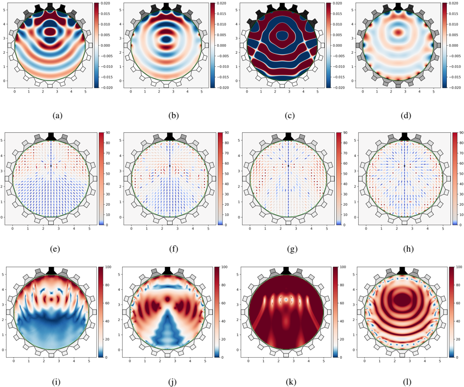
The image presents a composite figure consisting of twelve subplots (arranged in a 3x4 grid) that visualize data from a circular transducer array. Each subplot displays a different aspect of the data, including pressure fields, vector fields, and intensity plots. The subplots are labeled (a) through (l). The circular array is represented by a ring with small rectangular elements around its circumference.
### Components/Axes
**General Components:**
* **Circular Transducer Array:** A ring with small rectangular elements around the circumference, representing the transducers. A single larger transducer is positioned at the top of the circle.
* **Cartesian Axes:** Each subplot has x and y axes ranging from 0 to 5.
* **Color Scales:** Several subplots use color scales to represent data values. These scales are located on the right side of the respective subplots.
**Specific Subplot Details:**
* **(a), (b), (c), (d):** These subplots display pressure fields using a color scale ranging from approximately -0.020 to 0.020. Red indicates positive pressure, blue indicates negative pressure, and white indicates zero pressure.
* **(e), (f), (g), (h):** These subplots display vector fields overlaid on a circular area. The vectors indicate the direction and magnitude of a field. A color scale on the right ranges from 0 to 90, presumably representing the magnitude of the vectors.
* **(i), (j), (k), (l):** These subplots display intensity plots using a color scale ranging from 0 to 100. Red indicates high intensity, and blue indicates low intensity.
### Detailed Analysis
**Subplots (a), (b), (c), (d): Pressure Fields**
* **Color Scale:** Ranges from -0.020 (blue) to 0.020 (red).
* **Trend:** These plots show spatial variations in pressure.
* **(a):** Shows a pattern with alternating red and blue regions, suggesting wave-like behavior.
* **(b):** Shows a central red region surrounded by blue regions.
* **(c):** Shows concentric rings of alternating red and blue.
* **(d):** Shows a pattern similar to (a) but with a different spatial arrangement.
**Subplots (e), (f), (g), (h): Vector Fields**
* **Color Scale:** Ranges from 0 (blue) to 90 (red).
* **Trend:** These plots show the direction and magnitude of a vector field.
* **(e):** Vectors generally point away from the top transducer.
* **(f):** Vectors show a more complex pattern with some pointing inward and some outward.
* **(g):** Vectors are primarily directed downwards.
* **(h):** Vectors show a more uniform distribution with varying directions.
**Subplots (i), (j), (k), (l): Intensity Plots**
* **Color Scale:** Ranges from 0 (blue) to 100 (red).
* **Trend:** These plots show the spatial distribution of intensity.
* **(i):** Shows high intensity near the top transducer, decreasing towards the bottom.
* **(j):** Shows a focused region of high intensity in the center.
* **(k):** Shows several distinct regions of high intensity radiating from the top.
* **(l):** Shows concentric rings of high intensity.
### Key Observations
* The circular transducer array is a common element across all subplots.
* The color scales provide a quantitative measure of the data being visualized.
* The different subplots represent different aspects of the data, such as pressure, vector direction/magnitude, and intensity.
* The spatial patterns vary significantly across the subplots, indicating different operating conditions or data processing methods.
### Interpretation
The composite figure likely represents different modes or configurations of the circular transducer array. The pressure fields, vector fields, and intensity plots provide complementary information about the array's behavior. The variations in spatial patterns suggest that the array can be configured to generate different types of acoustic fields. The data could be used to optimize the array's performance for specific applications, such as medical imaging, non-destructive testing, or acoustic manipulation. The different subplots likely correspond to different driving frequencies, phase delays, or transducer configurations.