TECHNICAL ASSET FINGERPRINT
a01c98589c5b810c2a28ed37
Click to view fullscreen
Press ESC or click to close
FOUND IN PAPERS
EXPERT: gemini-2.5-flash-free VERSION 2
RUNTIME: google-free/gemini-2.5-flash
INTEL_VERIFIED
## Multi-Panel Field Visualizations in a Circular Domain
### Overview
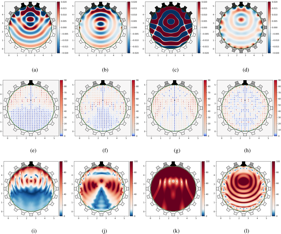
This image presents a grid of twelve sub-plots, arranged in three rows and four columns, labeled (a) through (l). Each sub-plot visualizes a field within a circular domain, which is outlined in green. Surrounding this circular domain are 18 external elements, likely transducers or sensors: two black trapezoidal shapes positioned at the top-center, and 16 grey trapezoidal shapes distributed around the remaining circumference. The plots are broadly categorized into three types based on their colorbar ranges and visual elements: scalar fields with signed values (a-d), scalar fields with superimposed vector fields (e-h), and scalar fields with non-negative values (i-l).
### Components/Axes
All sub-plots share common structural elements:
* **X-axis**: Labeled with numerical markers 0, 1, 2, 3, 4, 5, extending horizontally across the bottom of each circular domain.
* **Y-axis**: Labeled with numerical markers 1, 2, 3, 4, 5, extending vertically along the left side of each circular domain.
* **Circular Domain**: An inner region bounded by a thin green circular line, representing the area where the fields are visualized.
* **External Elements**: 18 trapezoidal shapes are arranged around the outer edge of the circular domain. Two of these are colored black and are positioned at the very top, centered above the circular domain. The remaining 16 are grey and are evenly distributed around the rest of the circumference.
* **Sub-plot Labels**: Each sub-plot is labeled with a lowercase letter in parentheses, positioned below its respective plot (e.g., (a), (b), (c), etc.).
* **Colorbars/Legends**: Each group of four sub-plots (rows) shares a common vertical colorbar on its right side, indicating the range of values represented by the colors.
**Colorbar Details:**
* **Plots (a) - (d)**:
* Range: -0.020 (dark blue) to 0.020 (dark red).
* Markers: -0.020, -0.015, -0.010, -0.005, 0.000 (white/light blue), 0.005, 0.010, 0.015, 0.020.
* **Plots (e) - (h)**:
* Range: 10 (dark blue) to 90 (dark red).
* Markers: 10, 20, 30, 40, 50, 60, 70, 80, 90.
* **Plots (i) - (l)**:
* Range: 0 (dark blue) to 100 (dark red).
* Markers: 0, 20, 40, 60, 80, 100.
### Detailed Analysis
#### Scalar Fields with Signed Values (Plots a-d)
These plots use a diverging color scheme where blue represents negative values, red represents positive values, and white/light blue represents values near zero.
* **(a)**:
* **Trend**: Displays a complex wave pattern with diagonal symmetry. A horizontal blue band (negative values, approximately -0.010 to -0.015) is prominent around the y=3 level. Two distinct red lobes (positive values, approximately 0.010 to 0.015) are visible in the top-left and bottom-right quadrants, while two blue lobes (negative values, approximately -0.010 to -0.015) are in the top-right and bottom-left quadrants.
* **Values**: Peaks around ±0.015.
* **(b)**:
* **Trend**: Shows a clear concentric circular wave pattern. A central red circle (positive values, approximately 0.010 to 0.015) is surrounded by a blue ring (negative values, approximately -0.010 to -0.015), which is then enclosed by another red ring (positive values, approximately 0.005 to 0.010). The intensity generally decreases towards the outer edge.
* **Values**: Peaks around ±0.015.
* **(c)**:
* **Trend**: Exhibits a pattern of alternating vertical stripes. A strong central vertical blue band (negative values, approximately -0.015 to -0.020) is flanked by two dark red bands (positive values, approximately 0.015 to 0.020). Further out, blue bands appear. The pattern is symmetric about the vertical axis.
* **Values**: Peaks around ±0.020.
* **(d)**:
* **Trend**: Features a central red region (positive values, approximately 0.005 to 0.010), surrounded by an inner blue ring (negative values, approximately -0.005 to -0.010). The outer region displays a more complex arrangement of alternating red and blue lobes, suggesting a combination of radial and angular variations.
* **Values**: Peaks around ±0.010.
#### Scalar Fields with Vector Fields (Plots e-h)
These plots combine a heatmap with a sequential color scheme (blue for lower values, red for higher values) and superimposed blue arrows representing a vector field.
* **(e)**:
* **Heatmap Trend**: The top half of the circular domain (above y~3) is predominantly red (higher values, approximately 60-80), while the bottom half is predominantly blue (lower values, approximately 10-30). A horizontal transition zone is visible around y=3.
* **Vector Field Trend**: Blue arrows in the top half generally point downwards and slightly inwards towards the center. Arrows in the bottom half generally point upwards and slightly outwards. This indicates a flow pattern diverging from the bottom and converging towards the top, or vice-versa.
* **(f)**:
* **Heatmap Trend**: Similar to (e), with the top half red (approximately 60-80) and the bottom half blue (approximately 10-30). The horizontal transition appears slightly more defined.
* **Vector Field Trend**: The arrow pattern is very similar to (e), with downward-inward flow in the top and upward-outward flow in the bottom.
* **(g)**:
* **Heatmap Trend**: Again, the top half is red (approximately 60-80) and the bottom half is blue (approximately 10-30). The transition zone shows some central red extension downwards.
* **Vector Field Trend**: The arrow pattern is consistent with (e) and (f), showing a similar flow.
* **(h)**:
* **Heatmap Trend**: The top half is red (approximately 60-80) and the bottom half is blue (approximately 10-30). The transition appears smoother than in previous plots in this row.
* **Vector Field Trend**: The arrow pattern remains consistent with (e), (f), and (g), indicating a stable flow characteristic across these variations.
#### Scalar Fields with Non-Negative Values (Plots i-l)
These plots use a sequential color scheme where dark blue represents zero or very low values, and dark red represents the highest values.
* **(i)**:
* **Trend**: Features a strong red region (high values, approximately 80-100) in the top half, with complex, finger-like wave patterns extending downwards into the predominantly blue (low values, approximately 0-20) bottom half.
* **Values**: Ranges from 0 to 100.
* **(j)**:
* **Trend**: Shows a strong red region (high values, approximately 80-100) in the top half. A prominent V-shaped blue region (low values, approximately 0-20) extends upwards from the bottom-center, creating a distinct pattern symmetric about the vertical axis. The regions flanking the blue V-shape are red (approximately 60-80).
* **Values**: Ranges from 0 to 100.
* **(k)**:
* **Trend**: Characterized by highly concentrated red regions (high values, approximately 80-100) in the top half, forming multiple distinct lobes or "fingers" extending downwards. The entire circular domain is largely dominated by red, indicating high values throughout (approximately 60-100), with very little blue.
* **Values**: Predominantly high, ranging from 60 to 100.
* **(l)**:
* **Trend**: Displays a very clear and intense concentric circular wave pattern, similar to (b) but with non-negative values. A central intense red circle (high values, approximately 80-100) is surrounded by a dark blue ring (low values, approximately 0-20), followed by another intense red ring, and so on. The pattern shows distinct oscillations between high and low values.
* **Values**: Oscillates between 0-20 and 80-100.
### Key Observations
* **Consistent Setup**: All 12 plots share the same circular domain, axis ranges, and external transducer arrangement, suggesting they represent different states or measurements within the same system.
* **Distinct Field Types**: The three rows clearly differentiate between signed scalar fields, vector fields superimposed on scalar fields, and non-negative scalar fields, likely representing different physical quantities (e.g., pressure, velocity, intensity).
* **Symmetry and Patterns**: Many plots exhibit clear symmetry (e.g., (b), (c), (j), (l) show vertical or radial symmetry). Patterns range from simple concentric circles (b, l) to vertical stripes (c) and complex wave-like structures (a, i).
* **Directional Flow**: The vector fields (e-h) consistently show a flow pattern originating from the bottom and moving towards the top, or vice-versa, with a strong influence from the top-center region where the black transducers are located.
* **Energy Localization**: Plots (i-l) show regions of high energy (intense red) which are often localized or concentrated, particularly in the upper half of the domain.
### Interpretation
These visualizations likely represent acoustic or wave fields within a circular resonator or medium, possibly a fluid-filled cavity or a solid disk. The external trapezoidal elements are almost certainly transducers, with the two black ones at the top potentially acting as primary sources or receivers, given their distinct color and the observed field patterns.
* **Plots (a)-(d)**, with their signed values, could represent **acoustic pressure fields** or displacement fields, where positive and negative values indicate compression and rarefaction, or displacement in opposite directions. The variations between these plots might correspond to different resonant modes or excitation frequencies. For instance, (b) and (l) suggest radial modes, while (c) suggests a standing wave pattern.
* **Plots (e)-(h)**, combining a scalar field with a vector field, most likely depict **particle velocity fields** (vectors) superimposed on a scalar quantity like acoustic intensity or energy density. The consistent downward-inward/upward-outward flow in the vector fields, especially originating from the top, strongly suggests that the black transducers are acting as sources, driving the medium. The scalar field in these plots (red at top, blue at bottom) could represent the magnitude of the velocity or a related energy metric, indicating higher activity near the source.
* **Plots (i)-(l)**, with their non-negative values, are highly indicative of **acoustic intensity** or **energy density** fields. These quantities are always positive and represent the power flow or energy stored in the medium. The intense red regions highlight areas of high energy concentration. The concentric patterns in (l) further support the idea of wave propagation and energy distribution.
The overall set of plots provides a comprehensive view of how different physical quantities (pressure, velocity, intensity) behave under various conditions or modes within the circular domain, likely influenced by the specific arrangement and activation of the external transducers. The differences between the plots in each row could represent different excitation signals, frequencies, or phases, demonstrating the versatility of the system in generating diverse field patterns. The consistent flow in (e)-(h) points to a directional energy transfer, possibly for applications like focused ultrasound or acoustic manipulation.
DECODING INTELLIGENCE...