TECHNICAL ASSET FINGERPRINT
a01c98589c5b810c2a28ed37
Click to view fullscreen
Press ESC or click to close
FOUND IN PAPERS
EXPERT: gemini-2.5-flash-lite-free VERSION 1
RUNTIME: google-free/gemini-2.5-flash-lite
INTEL_VERIFIED
## Heatmaps and Vector Plots: Analysis of Circular Wave Phenomena
### Overview
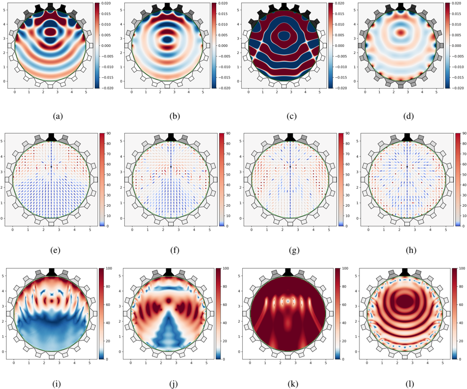
This image displays a collection of twelve plots, arranged in a 3x4 grid, labeled (a) through (l). The plots appear to visualize wave phenomena within a circular domain, characterized by a segmented outer boundary resembling a gear or a series of transducers. Plots (a) through (d) are heatmaps showing scalar field distributions. Plots (e) through (h) are vector plots, indicating direction and magnitude. Plots (i) through (l) are heatmaps, likely representing magnitudes or intensities. All plots share a common circular boundary and a coordinate system with axes ranging from 0 to 5.
### Components/Axes
**General Plot Structure:**
Each plot features a circular region of interest, surrounded by a segmented outer ring. A green circle delineates the primary area of analysis within each plot. The coordinate system for all plots has an x-axis and a y-axis, both ranging from 0 to 5.
**Plots (a) - (d): Heatmaps**
* **Colorbar:** Each of these plots has an associated colorbar on the right side, indicating a range from -0.020 to 0.020, with increments of 0.005. The color scale transitions from dark blue (negative values) through white (zero) to dark red (positive values).
* **Labels:** The colorbar is implicitly labeled as representing a scalar field value.
* **Axis Markers:** Both x and y axes are marked with numerical values from 0 to 5, with tick marks at integer and half-integer intervals.
**Plots (e) - (h): Vector Plots**
* **Colorbar:** Each of these plots has an associated colorbar on the right side, indicating a range from 0 to 90, with increments of 10. The color scale transitions from dark blue (low values) through lighter blues and reds to dark red (high values).
* **Vector Arrows:** Arrows are overlaid on the circular domain. The direction of each arrow indicates the direction of a vector quantity, and the length of the arrow is proportional to its magnitude.
* **Color of Arrows:** The color of the arrows corresponds to the magnitude indicated by the colorbar.
* **Labels:** The colorbar is implicitly labeled as representing the magnitude of a vector quantity.
* **Axis Markers:** Both x and y axes are marked with numerical values from 0 to 5, with tick marks at integer and half-integer intervals.
**Plots (i) - (l): Heatmaps**
* **Colorbar:** Each of these plots has an associated colorbar on the right side, indicating a range from 0 to 100, with increments of 10. The color scale transitions from dark blue (low values) through lighter blues and reds to dark red (high values).
* **Labels:** The colorbar is implicitly labeled as representing a scalar field value, likely intensity or magnitude.
* **Axis Markers:** Both x and y axes are marked with numerical values from 0 to 5, with tick marks at integer and half-integer intervals.
**Outer Ring Elements:**
All plots feature a segmented outer ring with dark gray and black elements. These appear to be discrete components or boundary conditions.
### Detailed Analysis
**Plots (a) - (d): Scalar Field Distributions**
* **(a)**: Shows a complex wave pattern with multiple nodes and antinodes. The pattern is roughly symmetrical about the vertical axis. Values range from approximately -0.020 (dark blue) to 0.020 (dark red). The central region exhibits a strong positive (red) and negative (blue) oscillation.
* **(b)**: Displays a more radially symmetric wave pattern, resembling concentric rings. The values are predominantly positive (red) in the center and negative (blue) further out, with a range from approximately -0.015 to 0.015.
* **(c)**: Exhibits a pattern with distinct lobes and nodal lines. There are clear regions of strong positive (red) and negative (blue) values, with a range from approximately -0.020 to 0.020. The pattern appears to have some rotational symmetry.
* **(d)**: Shows a simpler, more localized wave pattern, with a central positive (red) region and surrounding negative (blue) regions. The range is approximately -0.015 to 0.015.
**Plots (e) - (h): Vector Field Distributions**
* **(e)**: Displays a vector field with arrows predominantly pointing downwards in the upper half and upwards in the lower half, suggesting a flow or force. The magnitudes, indicated by color, are generally higher in the upper half (up to ~80, dark red) and lower in the lower half (around ~20-30, light blue/pink).
* **(f)**: Shows a similar overall flow pattern to (e), with downward vectors in the top and upward in the bottom. The magnitudes appear to be more uniformly distributed, with a range from approximately 20 to 70.
* **(g)**: Presents a vector field with a more complex directional pattern. Vectors in the upper region point mostly downwards, while vectors in the lower region are more varied, with some pointing upwards and others radially outwards. Magnitudes are generally moderate, ranging from about 20 to 60.
* **(h)**: Displays a vector field with vectors generally pointing downwards in the upper half and upwards in the lower half, similar to (e) and (f). The magnitudes are relatively low, mostly below 40, with a significant portion below 20.
**Plots (i) - (l): Intensity/Magnitude Heatmaps**
* **(i)**: Shows a pattern of high intensity (dark red, ~90-100) concentrated in the upper central region, with intensity decreasing towards the edges and bottom. There are distinct vertical striations of high intensity.
* **(j)**: Exhibits a broad central region of high intensity (dark red, ~90-100), with intensity decreasing towards the edges. The pattern is more diffuse than in (i), with a clear V-shape of high intensity pointing downwards.
* **(k)**: Displays a highly localized pattern of intense energy (dark red, ~90-100) concentrated in the upper central region, forming several distinct bright spots or peaks.
* **(l)**: Shows a pattern of concentric rings of high intensity (dark red, ~90-100) emanating from the center, with decreasing intensity further out. This pattern strongly suggests a radial wave propagation.
### Key Observations
* **Wave Patterns:** Plots (a)-(d) and (i)-(l) clearly visualize different wave modes or distributions within the circular domain. The patterns range from simple radial waves to complex nodal structures.
* **Vector Fields:** Plots (e)-(h) suggest directional quantities, possibly related to the propagation or forces associated with the waves. The magnitudes of these vectors vary significantly across the plots and within each plot.
* **Intensity Distribution:** Plots (i)-(l) highlight regions of high energy or amplitude. The localization and shape of these high-intensity regions vary considerably, indicating different underlying phenomena.
* **Symmetry:** Some plots exhibit clear symmetry (e.g., radial symmetry in (b) and (l)), while others show more complex or asymmetric patterns.
* **Outer Ring Influence:** The segmented outer ring is a consistent feature across all plots, suggesting it plays a role in the boundary conditions or excitation of the phenomena being visualized.
### Interpretation
The collection of plots appears to represent simulations or experimental measurements of wave phenomena within a confined circular geometry, possibly a resonator or a transducer array.
* **Plots (a)-(d)** likely depict the spatial distribution of a scalar field, such as pressure, displacement, or electric potential, at different frequencies or modes. The distinct patterns suggest the excitation of various resonant modes within the circular cavity. For instance, plot (b) and (l) show radial modes, while (a) and (c) show more complex modes with nodal lines.
* **Plots (e)-(h)** are vector fields, which could represent the flow of energy, particle velocity, or force vectors associated with the waves. The varying magnitudes and directions suggest different physical processes at play. For example, the downward/upward flow in (e)-(h) might indicate energy transport or a driving mechanism.
* **Plots (i)-(l)** are likely heatmaps of the squared magnitude of the scalar field or the intensity of the wave. The concentration of high intensity in specific regions (e.g., the bright spots in (k) or the concentric rings in (l)) indicates where the wave energy is most pronounced. The V-shaped high-intensity region in (j) and the vertical striations in (i) suggest specific wave interference or confinement effects.
The overall presentation suggests an investigation into the behavior of waves in a circular system, possibly exploring different excitation methods or boundary conditions represented by the outer ring. The combination of scalar field, vector field, and intensity plots provides a comprehensive view of the wave dynamics. The distinct patterns observed across the different plots likely correspond to different modes of oscillation or propagation within the circular domain.
DECODING INTELLIGENCE...