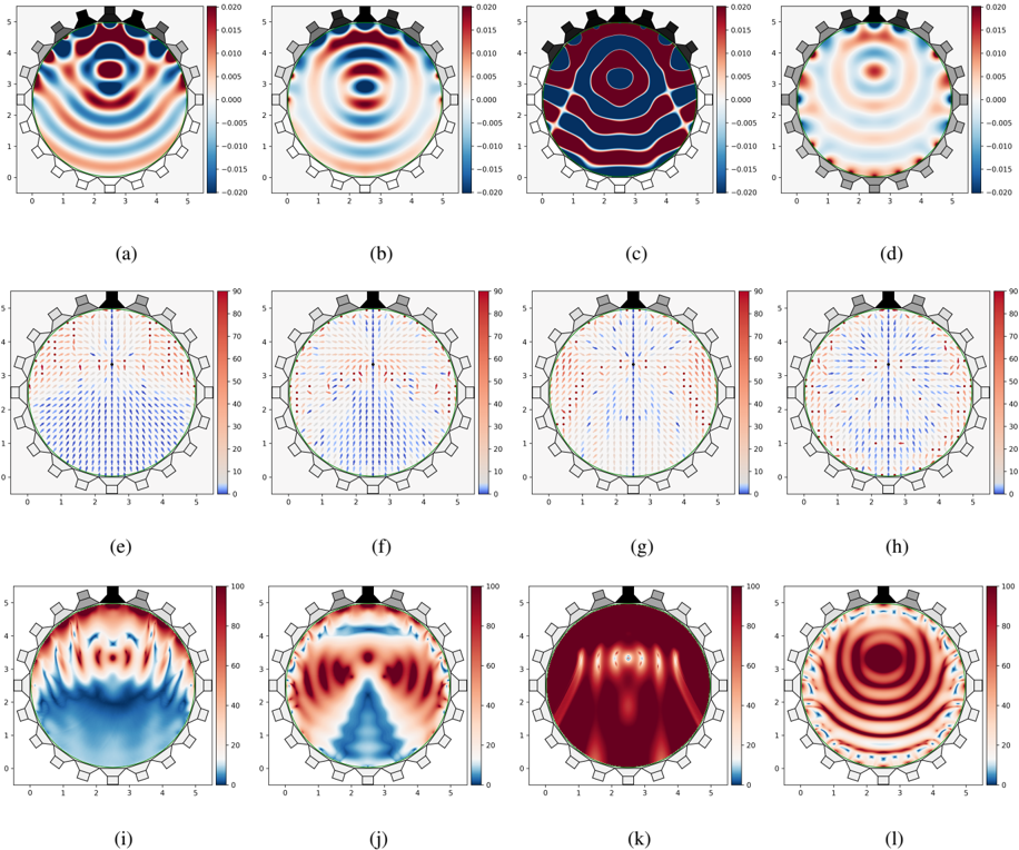
\n ## Heatmaps: Wave Propagation Simulations ### Overview The image presents a 4x3 grid of heatmaps, each representing a simulation of wave propagation within a circular domain with a gear-shaped obstacle at the top center. Each heatmap visualizes a different aspect of the wave field, likely at different times or with different parameters. The color scales vary between the top row (a-d) and the bottom two rows (e-l), indicating different physical quantities being represented. ### Components/Axes Each heatmap shares the following characteristics: * **Shape:** Circular domain with a gear-shaped obstacle. * **Axes:** Both x and y axes range from approximately 0 to 5, with tick marks at intervals of 1. * **Colorbar:** Each heatmap has a colorbar on the right side, representing the value of the quantity being visualized. * **Labels:** Each heatmap is labeled with a letter (a through l). The colorbars have different scales: * **Top Row (a-d):** Colorbar ranges from -0.020 to 0.020, with a color gradient from blue to red. * **Bottom Two Rows (e-l):** Colorbar ranges from 0 to 100, with a color gradient from blue to red. ### Detailed Analysis or Content Details **Top Row (a-d):** These heatmaps show wave patterns with both positive and negative values, indicated by the blue and red colors respectively. The patterns appear to be circular waves emanating from a central source. * **(a):** Concentric circular wave pattern. Values range from approximately -0.015 to 0.015. * **(b):** Similar to (a), but with a slightly distorted wave pattern. Values range from approximately -0.015 to 0.015. * **(c):** Wave pattern with more pronounced distortion due to the gear-shaped obstacle. Values range from approximately -0.015 to 0.015. * **(d):** Wave pattern with a more complex interference pattern. Values range from approximately -0.015 to 0.015. **Second Row (e-h):** These heatmaps show wave patterns with only positive values, indicated by the blue to red color gradient. The patterns appear to represent the amplitude or intensity of the wave. * **(e):** Wave pattern with a central maximum and decreasing intensity towards the edges. Values range from approximately 0 to 80. * **(f):** Wave pattern with multiple local maxima and minima. Values range from approximately 0 to 80. * **(g):** Wave pattern with a more complex interference pattern. Values range from approximately 0 to 80. * **(h):** Wave pattern with a central maximum and a ring-shaped region of high intensity. Values range from approximately 0 to 80. **Third Row (i-l):** These heatmaps also show wave patterns with only positive values, similar to the second row. * **(i):** Wave pattern with a highly distorted shape due to the gear-shaped obstacle. Values range from approximately 0 to 100. * **(j):** Wave pattern with a complex interference pattern and multiple local maxima. Values range from approximately 0 to 100. * **(k):** Wave pattern with a concentrated region of high intensity. Values range from approximately 0 to 100. * **(l):** Wave pattern with a ring-shaped region of high intensity. Values range from approximately 0 to 100. ### Key Observations * The top row (a-d) represents a quantity that can be both positive and negative, likely related to the phase or velocity potential of the wave. * The bottom two rows (e-l) represent a quantity that is always positive, likely related to the amplitude or energy density of the wave. * The gear-shaped obstacle significantly affects the wave patterns, causing diffraction and interference. * The wave patterns change over time or with different parameters, as evidenced by the differences between the heatmaps. * The maximum values in the bottom two rows are generally higher than those in the top row, suggesting that the amplitude or energy density of the wave is higher than the phase or velocity potential. ### Interpretation The image demonstrates simulations of wave propagation in a complex medium. The gear-shaped obstacle acts as a scattering object, causing the waves to diffract and interfere with each other. The different heatmaps likely represent snapshots of the wave field at different times or with different parameters, such as the frequency or amplitude of the wave. The color scales indicate the magnitude of the quantity being visualized, with red representing higher values and blue representing lower values. The variations in the wave patterns suggest that the system is sensitive to the shape and position of the obstacle, as well as the properties of the wave itself. This type of simulation could be used to study a variety of phenomena, such as sound propagation in a room with obstacles, electromagnetic wave scattering from a complex object, or water wave propagation around a breakwater. The differences between the top and bottom rows suggest that the simulations are tracking both the phase and amplitude of the wave, providing a more complete picture of the wave field. The outliers in the bottom row (i-l) suggest that the wave energy is being concentrated in certain regions due to the obstacle.