## Heatmaps and Vector Field Visualizations: Flow Patterns Around a Circular Domain
### Overview
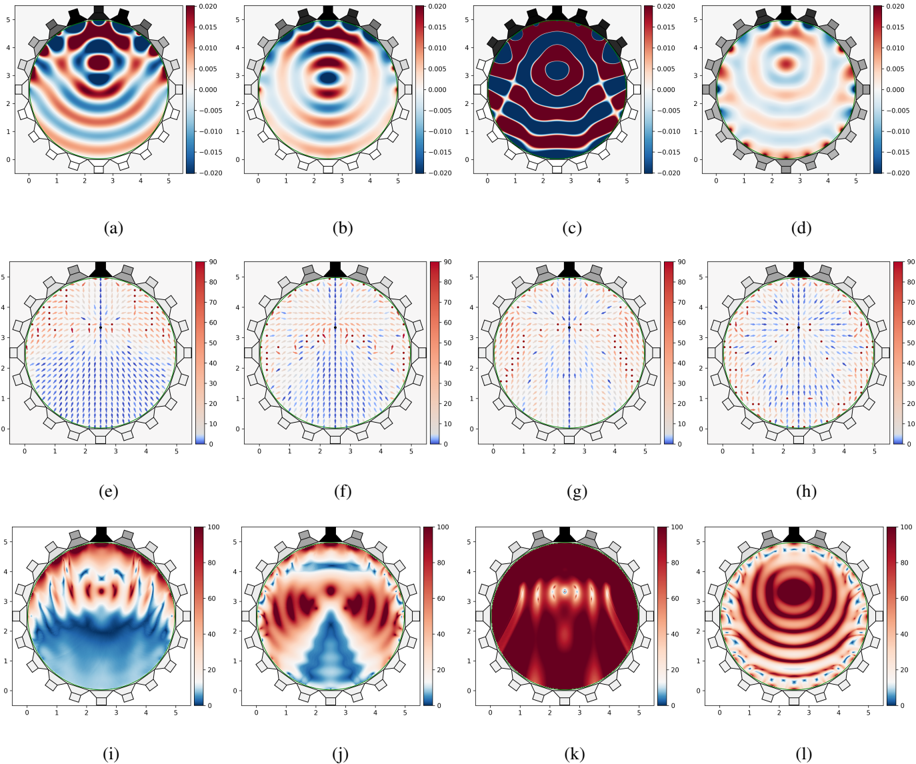
The image contains 12 subplots (a)-(l) depicting fluid dynamics simulations of flow patterns and pressure distributions around a circular domain with boundary conditions. Each subplot uses color gradients and vector fields to represent scalar quantities (e.g., pressure) and vector quantities (e.g., velocity direction/magnitude). The circular domain is bounded by gray square markers representing fixed boundary conditions.
---
### Components/Axes
- **Axes**:
- X-axis: 0–5 (linear scale)
- Y-axis: 0–5 (linear scale)
- Circular domain centered at (2.5, 2.5) with radius ~2.5 units.
- **Legends**:
- Color scales vary per subplot:
- Subplots (a)-(d): -0.020 to 0.020 (pressure/velocity magnitude).
- Subplots (e)-(h): 0 to 90 (velocity magnitude).
- Subplots (i)-(l): 0 to 100 (pressure/velocity magnitude).
- Arrows in vector fields (e)-(h) indicate direction and magnitude.
- **Boundary Conditions**: Gray squares along the circular perimeter (fixed walls or no-slip boundaries).
---
### Detailed Analysis
#### Subplots (a)-(d): Scalar Fields (Pressure/Velocity Magnitude)
- **(a)**: Central vortex with concentric pressure gradients. Red (high pressure) at the center transitions to blue (low pressure) at the edges.
- **(b)**: Spiral flow pattern with alternating high/low pressure regions.
- **(c)**: Alternating banded structure with sharp transitions between red and blue.
- **(d)**: Central vortex with radial streaks, suggesting turbulent flow.
#### Subplots (e)-(h): Vector Fields (Velocity Direction/Magnitude)
- **(e)**: Radial outward flow with uniform arrow density.
- **(f)**: Flow separation at the top boundary, creating recirculation zones.
- **(g)**: Symmetric flow with minimal deviation from the centerline.
- **(h)**: Complex flow with vortices and directional streaks.
#### Subplots (i)-(l): High-Magnitude Scalar Fields
- **(i)**: Sharp pressure gradient with a central low-pressure zone (blue) and high-pressure regions (red).
- **(j)**: Symmetric flow with a central vortex and radial pressure waves.
- **(k)**: High-pressure regions (red) dominate, with a central low-pressure zone.
- **(l)**: Concentric pressure waves resembling shock waves or acoustic patterns.
---
### Key Observations
1. **Flow Separation**: Subplots (f) and (h) show boundary-layer separation, indicated by reversed flow directions near the top boundary.
2. **Vortices**: Central vortices appear in (a), (d), (j), and (l), with varying intensity and structure.
3. **Pressure Gradients**: Subplots (i) and (k) exhibit extreme pressure contrasts, suggesting high-speed flow or shock interactions.
4. **Symmetry**: Subplots (e), (g), and (l) display axisymmetric flow, while (b) and (c) show asymmetric patterns.
---
### Interpretation
These visualizations likely represent computational fluid dynamics (CFD) simulations of flow around a circular object (e.g., a cylinder or sphere). The variations in flow patterns suggest differences in:
- **Reynolds Number**: Higher Reynolds numbers (turbulent flow) may explain the complex vortices in (d), (h), and (l).
- **Boundary Conditions**: Fixed walls (gray squares) influence flow separation and recirculation (e.g., (f)).
- **Flow Regimes**: Subplots (a)-(d) may represent laminar flow, while (e)-(h) and (i)-(l) show transitional/turbulent regimes.
The pressure distributions (red/blue gradients) correlate with velocity magnitudes (arrow lengths in vector fields), indicating regions of acceleration/deceleration. For example, the central low-pressure zones in (a), (j), and (k) align with high-velocity regions, consistent with Bernoulli’s principle.
The simulations could inform aerodynamic design, turbulence modeling, or boundary-layer control strategies. Outliers like the sharp pressure waves in (l) may represent unsteady flow phenomena or numerical artifacts requiring further validation.