## [Chart Type]: Comparative Line Charts - Algorithm Performance
### Overview
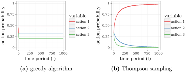
The image displays two side-by-side line charts comparing the performance of two different algorithms over time. The charts plot the "action probability" for three distinct actions (action 1, action 2, action 3) across 1000 time periods. The left chart (a) illustrates the behavior of a "greedy algorithm," while the right chart (b) shows the behavior of "Thompson sampling."
### Components/Axes
**Common Elements (Both Charts):**
* **X-Axis:** Labeled "time period (t)". The scale runs from 0 to 1000, with major tick marks at 0, 250, 500, 750, and 1000.
* **Y-Axis:** Labeled "action probability". The scale runs from 0 to 1, with major tick marks at 0, 0.25, 0.50, 0.75, and 1.
* **Legend:** Positioned to the right of each chart's plot area. It is titled "variable" and contains three entries:
* `action 1` - Represented by a red line.
* `action 2` - Represented by a blue line.
* `action 3` - Represented by a green line.
**Chart-Specific Labels:**
* **Chart (a):** Sub-caption below the plot reads "(a) greedy algorithm".
* **Chart (b):** Sub-caption below the plot reads "(b) Thompson sampling".
### Detailed Analysis
**Chart (a): Greedy Algorithm**
* **Trend Verification:** All three lines are perfectly horizontal and flat from time period 0 to 1000. This indicates the action probabilities are static and do not change over time.
* **Data Points (Approximate):**
* **Action 1 (Red Line):** Maintains a constant probability of approximately **0.47**.
* **Action 2 (Blue Line):** Maintains a constant probability of approximately **0.33**.
* **Action 3 (Green Line):** Maintains a constant probability of approximately **0.20**.
* **Spatial Grounding:** The lines are stacked vertically in the order Red (top), Blue (middle), Green (bottom) for the entire duration.
**Chart (b): Thompson Sampling**
* **Trend Verification:** The lines show dynamic, converging trends.
* The red line (action 1) slopes sharply upward initially and then asymptotically approaches 1.
* The blue line (action 2) slopes downward, approaching 0.
* The green line (action 3) slopes downward more steeply than the blue line, also approaching 0.
* **Data Points (Approximate):**
* **Action 1 (Red Line):** Starts at ~0.33 at t=0. Rises rapidly, crossing 0.75 by t≈150, and appears to exceed 0.95 by t=1000.
* **Action 2 (Blue Line):** Starts at ~0.33 at t=0. Declines steadily, falling below 0.1 by t≈400 and approaching near-zero by t=1000.
* **Action 3 (Green Line):** Starts at ~0.33 at t=0. Declines more rapidly than the blue line, falling below 0.1 by t≈200 and approaching near-zero by t=1000.
* **Spatial Grounding:** The lines start clustered near the same point (~0.33) at t=0. They immediately diverge, with the red line moving to the top of the chart and the blue and green lines moving to the bottom.
### Key Observations
1. **Fundamental Behavioral Contrast:** The greedy algorithm exhibits **static, fixed probabilities**, while Thompson sampling exhibits **dynamic, adaptive probabilities** that change dramatically over time.
2. **Convergence:** Thompson sampling demonstrates clear convergence, with the probability of one action (action 1) dominating and approaching certainty (1.0), while the probabilities of the other two actions diminish toward zero.
3. **Initial Conditions:** Both algorithms appear to start with similar initial probability distributions (roughly 0.47/0.33/0.20 for greedy and an initial cluster near 0.33 for Thompson sampling), but their evolution is completely different.
4. **Learning Signal:** The shape of the curves in the Thompson sampling chart suggests a learning process where the algorithm is identifying and exploiting the most rewarding action over time.
### Interpretation
This visualization contrasts two fundamental approaches in decision-making under uncertainty, likely within a multi-armed bandit or reinforcement learning context.
* **Greedy Algorithm (Chart a):** The flat lines suggest this algorithm has made a single, initial allocation of probabilities and never updates them. It is not learning from experience. The specific probabilities (0.47, 0.33, 0.20) may reflect a prior belief or a one-time optimization, but the algorithm is "stuck" in this configuration, regardless of the rewards it might be receiving. This represents a **non-adaptive, potentially suboptimal strategy**.
* **Thompson Sampling (Chart b):** The converging curves are the hallmark of a **successful learning algorithm**. Thompson sampling is a probabilistic algorithm that maintains a belief (a probability distribution) about which action is best. As it gathers more data (rewards) over time, it updates these beliefs. The chart shows this process in action: the algorithm quickly becomes increasingly confident that "action 1" is the optimal choice, allocating nearly all probability mass to it. The rapid initial change indicates efficient learning from early trials.
**Underlying Message:** The image powerfully argues for the superiority of adaptive, probabilistic methods like Thompson sampling over static, greedy approaches in sequential decision problems. It visually demonstrates how an intelligent algorithm can converge on an optimal policy through interaction with its environment, while a greedy algorithm remains stagnant. The "Peircean" abductive inference is that the environment likely has one action (action 1) that yields a higher reward than the others, and Thompson sampling has successfully inferred this fact through experimentation.