## Line Plots: Probability vs. α for Different γ Values
### Overview
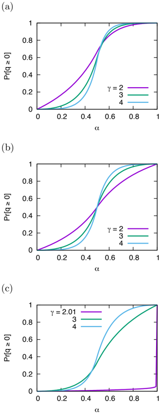
The image contains three vertically stacked line plots, labeled (a), (b), and (c). Each plot displays the relationship between a parameter `α` (x-axis) and a probability measure (y-axis) for different values of a parameter `γ`. The plots are rendered in a standard scientific style with black axes, tick marks, and colored lines.
### Components/Axes
**Common Elements:**
* **X-axis (All Plots):** Labeled `α`. The scale runs from 0 to 1, with major tick marks at intervals of 0.2 (0, 0.2, 0.4, 0.6, 0.8, 1).
* **Y-axis (All Plots):** The scale runs from 0 to 1, with major tick marks at intervals of 0.2 (0, 0.2, 0.4, 0.6, 0.8, 1).
* **Legends:** Each plot contains a legend in the top-left quadrant, associating line colors with specific `γ` values.
* **Line Colors:** Purple, Green, and Blue are used consistently across plots for different `γ` values.
**Plot-Specific Details:**
* **Plot (a):**
* **Y-axis Label:** `P(q = 0)`
* **Legend:** Located in the top-left. Entries: `γ = 2` (Purple line), `3` (Green line), `4` (Blue line).
* **Plot (b):**
* **Y-axis Label:** `P(q ≥ 0)`
* **Legend:** Located in the top-left. Entries: `γ = 2` (Purple line), `3` (Green line), `4` (Blue line).
* **Plot (c):**
* **Y-axis Label:** `P(q ≥ 0)`
* **Legend:** Located in the top-left. Entries: `γ = 2.01` (Purple line), `3` (Green line), `4` (Blue line).
### Detailed Analysis
**Trend Verification & Data Points:**
* **Plot (a) - `P(q = 0)` vs. `α`:**
* **Trend:** All three curves are sigmoidal (S-shaped), starting at 0 for `α=0` and saturating at 1 for `α=1`. The steepness of the transition increases with `γ`.
* **Purple Line (`γ=2`):** The shallowest curve. It begins rising immediately from `α=0`. It crosses the 0.5 probability mark at approximately `α ≈ 0.45`.
* **Green Line (`γ=3`):** Intermediate steepness. It remains near 0 until `α ≈ 0.2`, then rises sharply. It crosses 0.5 at approximately `α ≈ 0.5`.
* **Blue Line (`γ=4`):** The steepest curve. It stays very close to 0 until `α ≈ 0.3`, then exhibits the sharpest rise. It crosses 0.5 at approximately `α ≈ 0.52`.
* **Plot (b) - `P(q ≥ 0)` vs. `α`:**
* **Trend:** All curves increase from 0 to 1. The curves for `γ=3` and `γ=4` cross each other.
* **Purple Line (`γ=2`):** A smooth, concave-down curve. It rises steadily, crossing 0.5 at `α ≈ 0.5`.
* **Green Line (`γ=3`):** Starts lower than the purple line for `α < 0.5`, crosses it near `α ≈ 0.5`, and ends higher for `α > 0.5`. It crosses 0.5 at `α ≈ 0.5`.
* **Blue Line (`γ=4`):** Starts the lowest for `α < 0.5`, crosses both other lines near `α ≈ 0.5`, and becomes the highest for `α > 0.5`. It crosses 0.5 at `α ≈ 0.5`.
* **Plot (c) - `P(q ≥ 0)` vs. `α`:**
* **Trend:** The curve for `γ=2.01` is dramatically different from the others, showing a near-binary transition.
* **Purple Line (`γ=2.01`):** Remains extremely close to 0 (approximately `P(q ≥ 0) < 0.05`) for almost the entire range of `α` from 0 to just below 1. At `α ≈ 1`, it jumps almost vertically to 1.
* **Green Line (`γ=3`):** Similar in shape to the `γ=3` line in plot (b). It begins rising noticeably around `α ≈ 0.3`, crosses 0.5 at `α ≈ 0.55`, and approaches 1 as `α` approaches 1.
* **Blue Line (`γ=4`):** Similar in shape to the `γ=4` line in plot (b). It begins rising later than the green line, crosses 0.5 at `α ≈ 0.52`, and approaches 1 more steeply.
### Key Observations
1. **Effect of γ:** Increasing `γ` generally makes the transition from probability 0 to 1 sharper and shifts the midpoint of the transition to slightly higher `α` values in plot (a). In plots (b) and (c), higher `γ` leads to a lower probability for `α < 0.5` and a higher probability for `α > 0.5`.
2. **Critical Threshold at γ ≈ 2:** Plot (c) reveals a dramatic change in behavior when `γ` is just above 2 (`γ=2.01`). The probability `P(q ≥ 0)` is suppressed to near zero for all `α < 1`, indicating a possible phase transition or critical point in the underlying system at `γ=2`.
3. **Crossover Point:** In plots (b) and (c), the curves for different `γ` values all intersect in a narrow region around `α ≈ 0.5`. This suggests `α=0.5` is a special point where the probability is largely independent of `γ` for the measured quantity `P(q ≥ 0)`.
4. **Difference Between Metrics:** The metric `P(q=0)` in (a) shows a smooth, ordered family of curves. The metric `P(q ≥ 0)` in (b) and (c) shows curves that cross and, for `γ` near 2, exhibit extreme behavior.
### Interpretation
These plots likely illustrate the behavior of a statistical or physical system where `q` is an order parameter or a state variable, `α` is a control parameter (like a probability or fraction), and `γ` is another system parameter (like an exponent or interaction strength).
* **Plot (a)** shows that the probability of the system being in the specific state `q=0` increases smoothly with `α`, and this transition becomes more abrupt as `γ` increases.
* **Plots (b) and (c)** measure the probability of the system being in any state where `q` is non-negative. The crossing of curves indicates a trade-off: for low `α`, a lower `γ` gives a higher probability of `q ≥ 0`, but for high `α`, a higher `γ` gives a higher probability.
* The most significant finding is the **singular behavior at γ=2.01** in plot (c). This suggests that `γ=2` is a critical value. For `γ` just above 2, the system is "locked" into a state where `q` is almost certainly negative (`P(q ≥ 0) ≈ 0`) unless `α` is pushed to its maximum value of 1, at which point the state flips completely. This is characteristic of a system with a sharp phase transition or a bifurcation point. The data implies that the underlying model or phenomenon undergoes a fundamental change in behavior at `γ=2`.