## Line Graphs: Probability Pr(q≥0) vs Parameter α for Different γ Values
### Overview
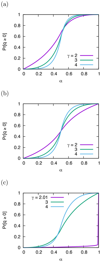
The image contains three vertically stacked line graphs (labeled a, b, c) showing the relationship between a parameter α (x-axis) and the probability Pr(q≥0) (y-axis) for three distinct values of γ (2, 3, 4). Each subplot uses the same color-coded legend: purple (γ=2), green (γ=3), and blue (γ=4). The graphs demonstrate how Pr(q≥0) evolves with α under different γ conditions.
### Components/Axes
- **X-axis**: Labeled α, ranging from 0 to 1 in all subplots.
- **Y-axis**: Labeled Pr(q≥0), ranging from 0 to 1 in all subplots.
- **Legends**: Positioned at the top-right of each subplot, explicitly mapping:
- Purple line → γ = 2
- Green line → γ = 3
- Blue line → γ = 4
- **Subplot Labels**: (a), (b), (c) for each graph.
### Detailed Analysis
#### Subplot (a)
- **Trend Verification**: All three lines (γ=2, 3, 4) start at (0,0) and asymptotically approach Pr(q≥0)=1 as α→1. The lines are closely spaced, with γ=2 (purple) consistently above γ=3 (green), which is above γ=4 (blue).
- **Key Data Points**:
- At α=0.2: Pr(q≥0) ≈ 0.1 (γ=2), 0.05 (γ=3), 0.03 (γ=4).
- At α=0.6: Pr(q≥0) ≈ 0.7 (γ=2), 0.65 (γ=3), 0.6 (γ=4).
- At α=0.9: Pr(q≥0) ≈ 0.95 (γ=2), 0.92 (γ=3), 0.88 (γ=4).
#### Subplot (b)
- **Trend Verification**: Lines cross near α=0.5. γ=2 (purple) starts below γ=3 (green) but overtakes it after α≈0.4. γ=4 (blue) remains the lowest throughout.
- **Key Data Points**:
- At α=0.3: Pr(q≥0) ≈ 0.2 (γ=2), 0.25 (γ=3), 0.15 (γ=4).
- At α=0.7: Pr(q≥0) ≈ 0.8 (γ=2), 0.7 (γ=3), 0.6 (γ=4).
#### Subplot (c)
- **Trend Verification**: γ=2 (purple) shows a delayed response, remaining near 0 until α≈0.8. γ=3 (green) and γ=4 (blue) rise sharply, with γ=4 consistently above γ=3.
- **Key Data Points**:
- At α=0.5: Pr(q≥0) ≈ 0.01 (γ=2), 0.4 (γ=3), 0.45 (γ=4).
- At α=0.9: Pr(q≥0) ≈ 0.99 (γ=2), 0.95 (γ=3), 0.97 (γ=4).
### Key Observations
1. **γ Dependency**: Higher γ values (3, 4) generally require larger α to achieve the same Pr(q≥0) compared to γ=2, except in subplot (b) where γ=2 overtakes γ=3.
2. **Threshold Behavior**: Subplot (c) suggests a critical α threshold (~0.8) for γ=2 to transition from near-zero to near-unity probability.
3. **Crossing Phenomenon**: Subplot (b) reveals a reversal in the γ=2 vs γ=3 relationship, indicating non-monotonic interactions between α and γ.
### Interpretation
The graphs illustrate how the probability Pr(q≥0) depends on the interplay between α and γ. In subplot (a), γ acts as a scaling factor, with higher γ requiring larger α to achieve the same probability. Subplot (b) introduces a non-linear interaction where γ=2 becomes more effective than γ=3 at intermediate α values, suggesting a competitive or compensatory mechanism. Subplot (c) highlights a critical α threshold for γ=2, implying a phase transition or tipping point behavior. These trends could reflect phenomena such as sensitivity thresholds in dynamical systems, resource allocation efficiency, or phase transitions in statistical mechanics, depending on the underlying model.