## Diagram: Neural Network Architecture ### Overview The image is a diagram illustrating the architecture of a neural network. It shows the flow of information from the input layer through multiple hidden layers to the output layer. The diagram highlights the connections between neurons in adjacent layers. ### Components/Axes * **Layers:** * Input Layer: Labeled "Input Layer" on the left. Contains nodes x1, x2, x3, ..., xp. Nodes are colored blue. * Hidden Layers: Labeled "Hidden Layers" at the top. Contains multiple layers labeled L1, L2, ..., Lm. Each hidden layer contains nodes h11, h12, h13, h14, ..., h1n1 for L1; h21, h22, h23, h24, ..., h2n2 for L2; and hm1, hm2, hm3, hm4, ..., hmnm for Lm. Nodes are colored green. * Output Layer: Labeled "Output Layer" on the right. Contains nodes o1, o2. Nodes are colored yellow. * **Connections:** * Connections between the input layer and the first hidden layer (L1) are blue. * Connections between hidden layers (L1 to L2, L2 to Lm) are green. * Connections between the last hidden layer (Lm) and the output layer are green. ### Detailed Analysis * **Input Layer:** * Nodes: x1, x2, x3, ..., xp. * Color: Blue. * Arrangement: Vertically stacked. * **Hidden Layer L1:** * Nodes: h11, h12, h13, h14, ..., h1n1. * Color: Green. * Arrangement: Vertically stacked. * **Hidden Layer L2:** * Nodes: h21, h22, h23, h24, ..., h2n2. * Color: Green. * Arrangement: Vertically stacked. * **Hidden Layer Lm:** * Nodes: hm1, hm2, hm3, hm4, ..., hmnm. * Color: Green. * Arrangement: Vertically stacked. * **Output Layer:** * Nodes: o1, o2. * Color: Yellow. * Arrangement: Vertically stacked. * **Connections:** * Each node in the input layer is connected to every node in the first hidden layer (L1). * Each node in each hidden layer is connected to every node in the subsequent hidden layer. * Each node in the last hidden layer (Lm) is connected to every node in the output layer. ### Key Observations * The diagram illustrates a fully connected neural network. * The number of nodes in each layer can vary. * The diagram uses color to differentiate the layers and connections. ### Interpretation The diagram represents a standard feedforward neural network architecture. The input layer receives the initial data, which is then processed through multiple hidden layers. Each hidden layer applies a series of transformations to the data, and the final output is produced by the output layer. The connections between the nodes represent the weights of the network, which are learned during the training process. The diagram highlights the flow of information and the interconnectedness of the network's components. The "..." notation indicates that the number of nodes in each layer can be variable and potentially large.

\n ## Diagram: Multi-Layer Perceptron (Neural Network) ### Overview The image depicts a diagram of a multi-layer perceptron, a type of artificial neural network. It illustrates the connections between input, hidden, and output layers, showcasing a feedforward network structure. The diagram is primarily conceptual, demonstrating the architecture rather than specific numerical data. ### Components/Axes The diagram consists of the following labeled components: * **Input Layer:** Labeled "Input Layer" at the top-left. Contains nodes labeled x₁, x₂, x₃, ..., xₚ. * **Hidden Layers:** Labeled "Hidden Layers" across the top-center. Specifically, layers L₁, L₂, ..., Lₘ are shown. * **Layer L₁:** Contains nodes labeled h₁₁, h₁₂, h₁₃, h₁₄, ..., h₁ₙ₁. * **Layer L₂:** Contains nodes labeled h₂₁, h₂₂, h₂₃, h₂₄, ..., h₂ₙ₂. * **Layer Lₘ:** Contains nodes labeled hₘ₁, hₘ₂, hₘ₃, hₘ₄, ..., hₘₙₘ. * **Output Layer:** Labeled "Output Layer" at the top-right. Contains nodes labeled o₁, o₂. * **Connections:** Gray lines represent connections between nodes in adjacent layers. These connections are weighted, but the weights are not explicitly shown. ### Detailed Analysis or Content Details The diagram shows a fully connected feedforward neural network. * **Input Layer:** The input layer has 'p' number of nodes, represented by x₁, x₂, x₃, and so on up to xₚ. * **Hidden Layers:** There are 'm' hidden layers. The first hidden layer (L₁) has 'n₁' nodes, the second (L₂) has 'n₂' nodes, and the last (Lₘ) has 'nₘ' nodes. * **Connections:** Each node in a given layer is connected to every node in the subsequent layer. This is indicated by the dense network of gray lines. * **Output Layer:** The output layer has two nodes, o₁ and o₂. ### Key Observations * The diagram illustrates a fully connected network, meaning every neuron in one layer is connected to every neuron in the next layer. * The number of layers and nodes per layer are variable, indicated by the use of subscripts (e.g., L₁, n₁, m). * The diagram does not provide any information about activation functions, learning rates, or other training parameters. * The diagram is a general representation and does not specify the specific application or task for which the network is designed. ### Interpretation The diagram represents a fundamental architecture in deep learning – the multi-layer perceptron. It demonstrates how input data is processed through multiple layers of interconnected nodes to produce an output. The connections between nodes represent weighted sums, and the hidden layers allow the network to learn complex, non-linear relationships in the data. The diagram highlights the core concept of feature extraction and transformation that occurs within a neural network. The absence of specific values suggests this is a conceptual illustration rather than a depiction of a trained network with defined weights and biases. The diagram is a blueprint for a computational model, not a record of its performance.

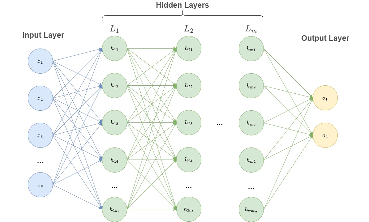
## Diagram: Artificial Neural Network Architecture ### Overview The image is a technical diagram illustrating the architecture of a feedforward artificial neural network (ANN), specifically a multi-layer perceptron (MLP). It visually represents the flow of data from an input layer, through one or more hidden layers, to an output layer. The diagram uses a standard node-and-edge notation where circles represent neurons (nodes) and lines represent weighted connections between them. ### Components/Axes The diagram is organized into three primary vertical sections, labeled from left to right: 1. **Input Layer** (Leftmost section, light blue nodes): * Label: "Input Layer" * Nodes: Labeled `x₁`, `x₂`, `x₃`, followed by an ellipsis (`...`), and ending with `xₚ`. This indicates an input vector of `p` dimensions. 2. **Hidden Layers** (Central section, light green nodes): * Main Label: "Hidden Layers" (centered above the section). * The section is subdivided into multiple layers, each with its own label: * Layer 1: Labeled `L₁`. Contains nodes labeled `h₁₁`, `h₁₂`, `h₁₃`, `h₁₄`, followed by an ellipsis (`...`), and ending with `h₁ₙ₁`. This indicates the first hidden layer has `n₁` neurons. * Layer 2: Labeled `L₂`. Contains nodes labeled `h₂₁`, `h₂₂`, `h₂₃`, `h₂₄`, followed by an ellipsis (`...`), and ending with `h₂ₙ₂`. This indicates the second hidden layer has `n₂` neurons. * Intermediate Layers: An ellipsis (`...`) is placed between Layer 2 and the final hidden layer, indicating the potential for additional hidden layers. * Final Hidden Layer (m-th layer): Labeled `Lₘ`. Contains nodes labeled `hₘ₁`, `hₘ₂`, `hₘ₃`, `hₘ₄`, followed by an ellipsis (`...`), and ending with `hₘₙₘ`. This indicates the m-th hidden layer has `nₘ` neurons. 3. **Output Layer** (Rightmost section, light yellow nodes): * Label: "Output Layer" * Nodes: Labeled `o₁` and `o₂`. This indicates the network produces a 2-dimensional output vector. **Connections (Edges):** * **Input to Hidden (L₁):** Blue lines connect every input node (`x₁` through `xₚ`) to every node in the first hidden layer (`h₁₁` through `h₁ₙ₁`). This represents a fully connected layer. * **Hidden to Hidden:** Green lines connect every node in one hidden layer to every node in the subsequent hidden layer (e.g., all nodes in `L₁` connect to all nodes in `L₂`). This pattern continues through all hidden layers. * **Hidden (Lₘ) to Output:** Green lines connect every node in the final hidden layer (`hₘ₁` through `hₘₙₘ`) to every output node (`o₁` and `o₂`). ### Detailed Analysis * **Network Topology:** The diagram depicts a fully connected, feedforward neural network. The flow of information is strictly from left (input) to right (output), with no cycles or backward connections. * **Scalability Notation:** The use of ellipses (`...`) in the input layer, between hidden layers, and within each hidden layer is a critical notational element. It explicitly shows that the network is generalized: * The input dimension `p` can be any positive integer. * The number of hidden layers `m` can be any positive integer (including `m=1` for a single hidden layer). * The number of neurons `n₁`, `n₂`, ..., `nₘ` in each hidden layer can vary independently. * **Node Labeling Convention:** The labeling follows a systematic pattern: * Input nodes: `xᵢ` where `i` is the feature index (1 to `p`). * Hidden nodes: `hₗₖ` where `l` is the layer index (1 to `m`) and `k` is the neuron index within that layer (1 to `nₗ`). * Output nodes: `oⱼ` where `j` is the output index (1 to 2 in this case). ### Key Observations 1. **Fully Connected Layers:** Every possible connection between adjacent layers is drawn, emphasizing that this is a dense network where each neuron receives input from all neurons in the previous layer. 2. **Generalized Architecture:** The diagram is not a specific instance but a template for a class of neural networks. The variables (`p`, `m`, `n₁`, `n₂`, ..., `nₘ`) allow it to represent networks of vastly different sizes and complexities. 3. **Color Coding:** A consistent color scheme is used to differentiate layer types: light blue for input, light green for hidden, and light yellow for output. The connection lines also follow a scheme: blue for input-to-first-hidden, and green for all subsequent hidden-to-hidden and hidden-to-output connections. 4. **Output Dimension:** The output layer has exactly two nodes (`o₁`, `o₂`), suggesting this specific template is for a network designed for a task with two outputs (e.g., binary classification with two output neurons, or regression with two target variables). ### Interpretation This diagram serves as a foundational schematic for understanding deep learning models. It visually communicates the core concepts of a multi-layer perceptron: * **Hierarchical Feature Learning:** The multiple hidden layers (`L₁` to `Lₘ`) suggest the network's ability to learn increasingly abstract representations of the input data. Early layers (`L₁`) might learn simple features, while deeper layers (`Lₘ`) combine them into complex patterns. * **Universal Approximation:** The structure, with at least one hidden layer and non-linear activation functions (implied but not shown), represents a model that, in theory, can approximate any continuous function given sufficient neurons (`nₗ`). The ellipses highlight that increasing `m` and `nₗ` increases the model's capacity. * **Parameterization:** The diagram implicitly represents a large set of learnable parameters: the weights associated with every drawn connection line and biases for every hidden and output neuron (biases are not visualized). The total number of parameters is determined by the values of `p`, `m`, and the `nₗ`'s. * **Task Specification:** The fixed output layer with two nodes indicates the network's final purpose is to produce a two-value output, framing the type of problem it is designed to solve. The input layer's variable size `p` shows it can accept feature vectors of different lengths. In essence, this image is a canonical representation of a deep neural network's "wiring diagram," abstracting away the specific mathematical operations (like weighted sums and activation functions) to focus on the architecture's topology and scalability.

## Neural Network Architecture Diagram ### Overview The image depicts a multi-layered artificial neural network with distinct input, hidden, and output layers. The architecture shows progressive transformations of input data through interconnected layers, culminating in output predictions. ### Components/Axes 1. **Input Layer** (Leftmost): - Labeled "Input Layer" - Contains nodes labeled x₁, x₂, ..., xₚ (p input features) - Blue circular nodes with blue connecting lines 2. **Hidden Layers** (Center): - Labeled "Hidden Layers" with sub-layers L₁ to Lₘ - Each layer contains nodes with hierarchical numbering: - L₁: h₁₁, h₁₂, ..., h₁ₙ₁ - L₂: h₂₁, h₂₂, ..., h₂ₙ₂ - ... - Lₘ: hₘ₁, hₘ₂, ..., hₘₙₘ - Green circular nodes with green connecting lines - Dense interconnections between nodes within and across layers 3. **Output Layer** (Rightmost): - Labeled "Output Layer" - Contains nodes labeled o₁, o₂ (2 output units) - Yellow circular nodes with green connecting lines from hidden layers 4. **Connections**: - Input → Hidden: Blue lines - Hidden → Hidden: Green lines - Hidden → Output: Green lines - No explicit activation functions or weights shown ### Detailed Analysis - **Layer Structure**: - Input layer (p nodes) → L₁ (n₁ nodes) → L₂ (n₂ nodes) → ... → Lₘ (nₘ nodes) → Output layer (2 nodes) - Node counts increase/decrease across layers (n₁ > n₂ > ... > nₘ suggested by diagram density) - **Color Coding**: - Input: Blue (nodes and connections) - Hidden: Green (nodes and connections) - Output: Yellow (nodes), Green connections - **Topology**: - Fully connected architecture (every node in one layer connects to every node in the next) - No skip connections or recurrent pathways visible ### Key Observations 1. The network has at least 3 layers (input, hidden, output) with potential for multiple hidden layers (L₁ to Lₘ) 2. Output layer has exactly 2 nodes, suggesting binary classification or regression task 3. Hidden layer node counts decrease progressively (n₁ > n₂ > ... > nₘ) 4. No explicit bias terms or activation functions depicted 5. All connections use consistent line styles within each connection type ### Interpretation This diagram represents a standard feedforward neural network architecture with: - **Input Processing**: Raw features (x₁...xₚ) transformed through multiple hidden layers - **Feature Hierarchy**: Each hidden layer (L₁...Lₘ) likely learns increasingly abstract representations - **Output Generation**: Final layer (Lₘ) produces predictions (o₁, o₂) through weighted combinations The architecture suggests a deep learning approach where: 1. Early layers (L₁) capture basic feature combinations 2. Middle layers (L₂...Lₘ₋₁) learn complex patterns 3. Final hidden layer (Lₘ) makes high-level abstractions for output The decreasing node count in hidden layers might indicate: - Regularization through reduced capacity in deeper layers - Computational efficiency considerations - Domain-specific feature hierarchy requirements The binary output (o₁, o₂) implies the network is designed for: - Binary classification (e.g., spam/not-spam) - Binary regression (e.g., yes/no prediction) - Multi-label classification with two primary outputs