## Line Graphs: Cumulative Normalized Loss vs. Fraction of Examples
### Overview
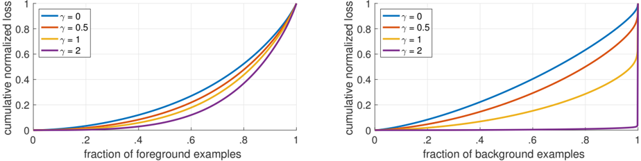
The image contains two side-by-side line graphs comparing cumulative normalized loss against the fraction of examples (foreground and background). Each graph displays four curves corresponding to different γ (gamma) values: 0, 0.5, 1, and 2. The curves illustrate how loss accumulates as the proportion of examples increases.
### Components/Axes
- **Left Graph (Foreground Examples)**:
- **X-axis**: "fraction of foreground examples" (0 to 1 in increments of 0.2).
- **Y-axis**: "cumulative normalized loss" (0 to 1 in increments of 0.2).
- **Legend**: Top-left, mapping γ values to colors:
- γ = 0: Blue
- γ = 0.5: Orange
- γ = 1: Yellow
- γ = 2: Purple
- **Right Graph (Background Examples)**:
- **X-axis**: "fraction of background examples" (0 to 1 in increments of 0.2).
- **Y-axis**: "cumulative normalized loss" (0 to 1 in increments of 0.2).
- **Legend**: Top-left, identical color coding as the left graph.
### Detailed Analysis
#### Left Graph (Foreground Examples)
- **γ = 0 (Blue)**: The curve starts at (0,0) and rises gradually, reaching ~0.8 at x=1.
- **γ = 0.5 (Orange)**: Steeper than γ=0, reaching ~0.85 at x=1.
- **γ = 1 (Yellow)**: Even steeper, reaching ~0.9 at x=1.
- **γ = 2 (Purple)**: The steepest curve, reaching ~0.95 at x=1.
- **Trend**: All curves start at the origin and end at (1,1), with higher γ values producing sharper increases in loss.
#### Right Graph (Background Examples)
- **γ = 0 (Blue)**: Starts at (0,0) and rises slowly, reaching ~0.6 at x=1.
- **γ = 0.5 (Orange)**: Steeper than γ=0, reaching ~0.7 at x=1.
- **γ = 1 (Yellow)**: Reaches ~0.8 at x=1.
- **γ = 2 (Purple)**: The steepest curve, reaching ~0.9 at x=1.
- **Trend**: Similar to the left graph, but all curves plateau below 1.0, with γ=2 approaching ~0.9.
### Key Observations
1. **Consistent γ Behavior**: Higher γ values consistently produce steeper curves in both graphs, indicating a direct relationship between γ and loss sensitivity.
2. **Asymmetry Between Foreground/Background**: For the same γ, the loss increase is more pronounced for foreground examples (left graph) than background examples (right graph).
3. **Convergence at x=1**: All curves reach 1.0 for foreground examples but plateau below 1.0 for background examples, suggesting a ceiling effect for background loss.
### Interpretation
The graphs demonstrate that:
- **γ Controls Sensitivity**: Higher γ values amplify the impact of example inclusion on cumulative loss, particularly for foreground data.
- **Imbalanced Impact**: Foreground examples drive loss more aggressively than background examples, even at the same γ. This could reflect class imbalance or differential weighting in the model.
- **Practical Implications**: Tuning γ may help balance loss contributions from foreground/background examples, critical for tasks like anomaly detection or imbalanced classification.
No outliers or anomalies are observed. The data suggests a systematic relationship between γ, example type, and loss accumulation.