## 3D Surface Plot: Relationship Between x₁, x₂, and True α - FE
### Overview
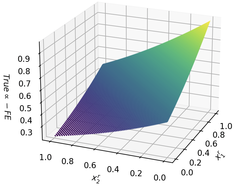
The image depicts a 3D surface plot visualizing the relationship between two input variables (x₁ and x₂) and a dependent variable labeled "True α - FE." The plot uses a color gradient (purple to yellow) to represent the magnitude of "True α - FE," with grid lines providing spatial context. The axes range from 0.0 to 1.0 for both x₁ and x₂, while "True α - FE" spans approximately 0.3 to 0.9.
---
### Components/Axes
1. **Axes Labels**:
- **X-axis (x₁)**: Labeled as "x₁," scaled from 0.0 to 1.0 in increments of 0.2.
- **Y-axis (x₂)**: Labeled as "x₂," scaled from 0.0 to 1.0 in increments of 0.2.
- **Z-axis (True α - FE)**: Labeled as "True α - FE," scaled from 0.3 to 0.9 in increments of 0.1.
2. **Grid Lines**:
- Gray grid lines span all three axes, creating a 3D lattice to contextualize the surface.
3. **Color Gradient**:
- The surface transitions from **purple** (low values) to **yellow** (high values), indicating the magnitude of "True α - FE."
---
### Detailed Analysis
1. **Surface Shape**:
- The surface forms a **diagonal ridge** from the bottom-left corner (x₁=0.0, x₂=0.0) to the top-right corner (x₁=1.0, x₂=1.0), suggesting a linear relationship between x₁, x₂, and "True α - FE."
- At (x₁=0.0, x₂=0.0), "True α - FE" ≈ 0.3 (purple).
- At (x₁=1.0, x₂=1.0), "True α - FE" ≈ 0.9 (yellow).
2. **Color Gradient**:
- Purple dominates the lower-left region (x₁ < 0.5, x₂ < 0.5), indicating lower "True α - FE" values.
- Yellow dominates the upper-right region (x₁ > 0.5, x₂ > 0.5), indicating higher "True α - FE" values.
- Intermediate values (green) appear along the diagonal ridge.
3. **Grid Line Interpretation**:
- The grid lines confirm the 3D structure, with horizontal lines representing x₁ and x₂, and vertical lines representing "True α - FE."
---
### Key Observations
1. **Linear Trend**:
- "True α - FE" increases linearly as both x₁ and x₂ increase, with the steepest gradient along the diagonal (x₁ = x₂).
2. **Color Correlation**:
- The color gradient aligns perfectly with the z-axis values, providing a visual cue for magnitude without numerical annotations.
3. **Boundary Values**:
- Minimum value (0.3) occurs at (0.0, 0.0).
- Maximum value (0.9) occurs at (1.0, 1.0).
---
### Interpretation
1. **Model Behavior**:
- The plot suggests that "True α - FE" is directly proportional to both x₁ and x₂. This could represent a simplified model where two input variables linearly influence a dependent variable (e.g., accuracy, error, or efficiency metric).
2. **Practical Implications**:
- Maximizing x₁ and x₂ (to 1.0) yields the highest "True α - FE," implying optimal performance or accuracy in the modeled system.
- The linear relationship simplifies predictive modeling, as no nonlinear interactions are observed.
3. **Anomalies**:
- No outliers or discontinuities are present, indicating a smooth, deterministic relationship.
4. **Design Choices**:
- The absence of a legend is compensated by the intuitive color gradient, which maps directly to the z-axis values.
- Grid lines enhance readability but may obscure fine details in the surface texture.
---
### Final Notes
This plot effectively communicates a linear, monotonic relationship between two inputs and a dependent variable. The use of color and grid lines aids in spatial grounding, though explicit numerical annotations on the surface could improve precision. The simplicity of the model suggests it may serve as a baseline for more complex analyses.