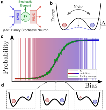
## Stochastic Neuron Diagram ### Overview The image illustrates the concept of a binary stochastic neuron (p-bit) and its behavior in terms of energy landscapes and probability distributions. It consists of four sub-figures: a schematic of the neuron (a), an energy landscape representation (b), a probability vs. bias plot (c), and three energy landscape examples corresponding to different bias levels (d). ### Components/Axes **Sub-figure a:** * **Elements:** * "BIAS" (blue rectangle): Input to the stochastic element. * "Stochastic Element" (green circle with "p" inside and an arrow): Represents the core stochastic processing unit. * "READ" (red rectangle): Output of the neuron. * **Arrows:** Indicate the flow of information. * **Label:** "p-bit: Binary Stochastic Neuron" - Describes the overall system. **Sub-figure b:** * **Axes:** * Vertical axis: "Energy" * **Curve:** A double-well potential energy landscape. * **Elements:** * Red and blue circles: Represent the two possible states of the p-bit. * "Noise" (gray double-headed arrow): Indicates the influence of noise on the system. * "Δ" (black bracket with label): Represents the energy barrier between the two states. * Dashed blue line: Represents the energy level of the lower well. **Sub-figure c:** * **Axes:** * Vertical axis: "Probability" (ranging from approximately 0 to 1). * Horizontal axis: "Bias" * **Data Series:** * Red vertical lines: Represent individual samples of the p-bit output. * Blue line: "tanh(Bias)" - Represents the theoretical probability based on the hyperbolic tangent function of the bias. It is approximately 0 for low bias values and 1 for high bias values. * Green line: "Rolling Average" - Represents the smoothed probability based on a rolling average of the p-bit output. It follows a sigmoidal curve, transitioning from approximately 0 to 1 as the bias increases. * **Background:** Gradient from red on the left to blue on the right, visually representing the influence of bias. * **Legend:** Located in the middle-right of the chart. **Sub-figure d:** * Three separate diagrams, each showing a double-well potential energy landscape similar to sub-figure b. * Each diagram has a red and blue circle representing the two possible states. * The relative depths of the two wells vary, representing different bias levels. ### Detailed Analysis **Sub-figure a:** * The diagram shows a simplified model of a stochastic neuron. The bias input influences the stochastic element, which then produces an output that can be read. **Sub-figure b:** * The energy landscape illustrates the two possible states of the p-bit as residing in the two wells. The "Noise" allows the p-bit to transition between these states. The energy barrier "Δ" determines the difficulty of switching states. **Sub-figure c:** * **Red Vertical Lines:** These lines are dense on the left side of the chart, indicating a high probability of being in the "red" state (approximately 0 probability). On the right side, the lines are dense, indicating a high probability of being in the "blue" state (approximately 1 probability). * **Blue Line (tanh(Bias)):** This line starts at approximately 0 for low bias values and gradually increases to approximately 1 for high bias values. * **Green Line (Rolling Average):** This line closely follows the trend of the blue line but is smoother due to the averaging effect. It starts at approximately 0 and increases to approximately 1 as the bias increases. * The three gray diamonds on the x-axis of the plot in (c) correspond to the three energy landscapes shown in (d). **Sub-figure d:** * The left diagram shows a landscape where the red state has a lower energy than the blue state, corresponding to a low bias. * The middle diagram shows a landscape where the two states have approximately equal energy, corresponding to an intermediate bias. * The right diagram shows a landscape where the blue state has a lower energy than the red state, corresponding to a high bias. ### Key Observations * The probability of the p-bit being in a particular state is directly related to the energy landscape and the applied bias. * The rolling average provides a smoothed representation of the p-bit's behavior, filtering out some of the noise. * The tanh(Bias) function provides a theoretical model for the probability, which is closely approximated by the rolling average. ### Interpretation The image demonstrates how a binary stochastic neuron operates. The bias input shifts the energy landscape, influencing the probability of the neuron being in one of two states. Noise allows the neuron to transition between these states, and the rolling average provides a stable estimate of the probability. The tanh(Bias) function provides a mathematical model for this behavior. The energy landscape diagrams in (d) visually represent how the bias affects the relative stability of the two states. This type of neuron can be used in various applications, such as probabilistic computing and neural networks.

## Diagram: Binary Stochastic Neuron & Probability Visualization ### Overview This image presents a conceptual diagram illustrating a binary stochastic neuron (p-bit) and its probabilistic behavior. It consists of a schematic of the neuron, a visualization of energy landscape with noise, and a probability plot showing the relationship between bias and probability. The bottom section shows the energy landscape at different bias values. ### Components/Axes The image is divided into four sections labeled (a), (b), (c), and (d). * **(a): Stochastic Element:** Shows a schematic of the neuron with "BIAS" inputs (blue arrows) and a "READ" output (red box). Inside the neuron is a circle labeled "p". Below this is the text "p-bit: Binary Stochastic Neuron". * **(b): Energy Landscape:** A plot of "Energy" vs. an unspecified axis. It depicts a double-well potential with two states represented by red and blue circles. An arrow labeled "Noise" indicates fluctuations between the states. A delta symbol (Δ) is present on the y-axis. * **(c): Probability vs. Bias Plot:** A plot of "Probability" (y-axis) vs. "Bias" (x-axis). It features three curves: * Red line: labeled "p" * Blue line: labeled "tanh (Bias)" * Green line: labeled "Rolling Average" The background is shaded with purple on the left and light blue on the right. Vertical lines are present throughout the plot. * **(d): Energy Landscapes at Different Biases:** Three energy landscapes are shown, each corresponding to a different bias value. The landscapes are similar to (b), but the position of the red and blue circles changes with increasing bias. Arrows connect these landscapes to the corresponding points on the x-axis of plot (c). ### Detailed Analysis or Content Details * **(a):** The "BIAS" inputs are represented as multiple blue arrows converging on the stochastic element. The output "READ" is a red box. The circle labeled "p" likely represents the probability of the neuron being in the active state. * **(b):** The energy landscape shows two potential wells. The red circle represents a state with lower energy, and the blue circle represents a state with higher energy. The "Noise" arrow indicates that the system can overcome the energy barrier and transition between states. The delta symbol (Δ) is not quantified. * **(c):** * The red line ("p") shows a highly fluctuating probability, with values oscillating between approximately 0 and 1. * The blue line ("tanh(Bias)") is a smooth, sigmoid-shaped curve. It starts near 0 for negative bias values, increases rapidly around bias = 0, and approaches 1 for positive bias values. * The green line ("Rolling Average") is a smoothed version of the red line, showing the overall trend. It also follows a sigmoid shape, similar to the blue line. * The purple shaded region on the left side of the plot corresponds to low probability values, while the light blue shaded region on the right corresponds to high probability values. * **(d):** As the bias increases (from left to right), the energy well corresponding to the blue circle deepens, while the energy well corresponding to the red circle shallows. This indicates that the system is more likely to be in the blue state at higher bias values. ### Key Observations * The stochastic neuron exhibits probabilistic behavior, with the probability of being in the active state (represented by "p") fluctuating significantly. * The "tanh(Bias)" curve provides a deterministic prediction of the probability based on the bias. * The rolling average smooths out the fluctuations and reveals the underlying trend. * The energy landscape visualization helps to understand the physical basis of the probabilistic behavior. ### Interpretation The diagram illustrates how a binary stochastic neuron can be modeled as a system with an energy landscape and noise. The bias controls the shape of the energy landscape, influencing the probability of the neuron being in different states. The noise allows the system to overcome energy barriers and transition between states, resulting in probabilistic behavior. The "tanh(Bias)" curve represents the deterministic component of the probability, while the fluctuations around this curve are due to the noise. The rolling average provides a way to estimate the underlying trend despite the noise. This model is relevant to understanding neural networks and other systems that exhibit stochastic behavior. The diagram suggests that the neuron's behavior is governed by a balance between deterministic bias and random noise. The energy landscape provides a visual metaphor for the decision-making process of the neuron.

## Multi-Panel Scientific Figure: p-bit (Binary Stochastic Neuron) Dynamics ### Overview The image is a four-panel scientific figure (labeled a, b, c, d) illustrating the components, energy landscape, probabilistic behavior, and state dynamics of a "p-bit" or binary stochastic neuron. The figure combines schematic diagrams, an energy potential plot, a probability vs. bias graph, and sequential energy landscape snapshots. ### Components/Axes **Panel a (Top Left):** * **Type:** Schematic diagram. * **Title/Label:** "p-bit: Binary Stochastic Neuron" (text below diagram). * **Components:** * A blue rectangular box labeled **"BIAS"** with two blue arrows pointing into it from the left. * A green circle containing the symbol **"p̃"** (p with a tilde). Above it is the label **"Stochastic Element"**. * A red rectangular box labeled **"READ"** with three red arrows pointing out to the right. * A green arrow connects the "BIAS" box to the "p̃" circle, and another green arrow connects the "p̃" circle to the "READ" box. **Panel b (Top Right):** * **Type:** Energy landscape diagram. * **Axes/Labels:** * Y-axis label: **"Energy"**. * A label **"Noise"** with two curved arrows above the central barrier, indicating fluctuations. * **Components:** * A double-well potential curve (black line). * A red dot in the left energy well. * A blue dot in the right energy well. * A vertical double-headed arrow labeled **"Δ"** (delta) indicating the energy difference between the two minima. * A dashed blue line shows a lower-energy path over the barrier. **Panel c (Center):** * **Type:** Line graph with background data distribution. * **Axes:** * Y-axis label: **"Probability"** (arrow pointing upward). * X-axis label: **"Bias"** (arrow pointing to the right). * **Legend (Bottom Right of Panel):** * **Green line:** Label **"p̃ᵢ"**. * **Red line:** Label **"tanh(Bias)"**. * **Blue line:** Label **"Rolling Average"**. * **Data Series & Trends:** * **Green Line (p̃ᵢ):** A highly noisy, sigmoidal curve that increases from near 0 to near 1 as Bias increases. It shows significant high-frequency fluctuations around a central trend. * **Red Line (tanh(Bias)):** A smooth, theoretical sigmoidal curve (hyperbolic tangent function) that closely follows the central trend of the noisy green line. It starts at 0, crosses 0.5 at a Bias value of approximately 0, and approaches 1. * **Blue Line (Rolling Average):** A step-like function that appears to be a binarized or thresholded version of the probability. It is near 0 for low Bias, jumps sharply to near 1 at a specific Bias threshold (approximately where the red/green curves cross 0.5), and remains near 1 for higher Bias. * **Background:** The plot area has a gradient background (pinkish-red on the left, purple on the right). Overlaid are numerous vertical lines: red lines concentrated on the left (low Bias) and blue lines concentrated on the right (high Bias), likely representing individual data points or samples. **Panel d (Bottom):** * **Type:** Series of three energy landscape diagrams. * **Components:** Each sub-panel shows a double-well potential (black curve) with a red dot and a blue dot. * **Left Sub-panel:** Red dot is deep in the left well; blue dot is high on the right slope, near the barrier. * **Middle Sub-panel:** Red dot is on the left slope, moving upward; blue dot is in the right well. * **Right Sub-panel:** Red dot is high on the left slope, near the barrier; blue dot is deep in the right well. * **Connection:** Dashed lines connect these three sub-panels to three specific points along the X-axis (Bias) of the graph in Panel c, indicating they represent system states at different bias values. ### Detailed Analysis * **Panel c Data Points (Approximate):** * The **red `tanh(Bias)` curve** crosses the 0.5 probability mark at a Bias value of approximately 0. * The **green `p̃ᵢ` curve** has a mean that follows the red curve but exhibits noise with an amplitude of roughly ±0.1 to ±0.2 probability across the transition region. * The **blue `Rolling Average`** transitions from ~0 to ~1 over a very narrow Bias range centered near 0. The transition appears almost vertical. * The **vertical background lines** suggest that for Bias << 0, the stochastic element (`p̃`) is almost always 0 (red lines), and for Bias >> 0, it is almost always 1 (blue lines). ### Key Observations 1. **Stochastic vs. Deterministic:** The core contrast is between the noisy, stochastic output of the p-bit (green line) and the smooth, deterministic `tanh` function (red line) which likely represents its expected value or a deterministic counterpart. 2. **Binarization:** The "Rolling Average" (blue line) demonstrates a sharp, threshold-like switching behavior, effectively converting the analog probability into a binary output (0 or 1). 3. **Energy Landscape Correspondence:** Panel d visually links the abstract probability curve to a physical analogy. As Bias increases (moving right on the x-axis in Panel c), the system's state (represented by the red and blue dots) shifts from favoring the left well (state 0) to favoring the right well (state 1). The "Noise" in Panel b enables transitions between these wells. 4. **Spatial Grounding:** The legend in Panel c is positioned in the bottom-right corner, clearly associating colors with data series. The connection lines from Panel d to Panel c are precise, mapping specific bias regimes to corresponding energy landscape configurations. ### Interpretation This figure explains the operational principle of a **binary stochastic neuron (p-bit)**, a component used in probabilistic computing and certain neural network models. * **What it demonstrates:** The p-bit's output is a stochastic binary value (0 or 1) whose **probability** of being 1 is a sigmoidal function of its input **Bias**. This is shown directly in Panel c. The `tanh` function provides a smooth, differentiable model for this probability, while the actual p-bit output (`p̃ᵢ`) is noisy. * **How elements relate:** The **Bias** (input) controls the shape of the **energy landscape** (Panel b). A positive bias lowers the energy of the "1" state (right well), making it more probable. **Noise** allows the system to occasionally overcome the energy barrier (Δ) between states, enabling stochastic switching. The **READ** operation (Panel a) samples this stochastic state. * **Underlying Mechanism:** The figure argues that the p-bit's behavior can be understood through a statistical physics lens: a particle (the system state) in a double-well potential, driven by an external field (Bias) and subject to thermal fluctuations (Noise). The sharp transition in the "Rolling Average" suggests that in a network or array of such p-bits, a collective, deterministic-like switching can emerge from many stochastic components. * **Notable Anomaly/Feature:** The extreme noisiness of the green `p̃ᵢ` line is not an error but a fundamental feature, highlighting the inherent randomness at the single-device level that the p-bit is designed to harness.

## Diagram: Binary Stochastic Neuron Model and Energy Landscape Analysis ### Overview The image presents a technical diagram of a binary stochastic neuron model (a), its energy landscape (b), a probability curve (c), and bias-dependent energy state visualizations (d). The components illustrate how stochastic neurons process inputs, manage noise, and convert bias into probabilistic outputs. ### Components/Axes **a. Binary Stochastic Neuron Diagram** - **Components**: - **p-bit**: Binary stochastic neuron (blue box) - **Stochastic Element**: Green circle labeled "Stochastic Element" - **READ**: Red box labeled "READ" - **Flow**: Arrows indicate input (p-bit → Stochastic Element) and output (Stochastic Element → READ). - **Labels**: - "p-bit: Binary Stochastic Neuron" (top-left) - "Stochastic Element" (green) - "READ" (red) **b. Energy Landscape** - **Axes**: Energy (y-axis, implicit) vs. Position (x-axis, implicit). - **Elements**: - Parabolic energy well with two states: - **Red dot**: High-energy state (unstable) - **Blue dot**: Low-energy state (stable) - **Noise**: Curved arrow labeled "Noise" between states. - **Δ**: Energy difference between states (vertical arrow). **c. Probability vs. Bias Graph** - **Axes**: - **y-axis**: Probability (labeled "Probability") - **x-axis**: Bias (labeled "Bias") - **Data Series**: - **Pi (red line)**: Probability of firing (P_i) - **tanh(Bias) (purple line)**: Sigmoid function of bias - **Rolling Average (green line)**: Smoothed version of Pi - **Legend**: Located at bottom-right, with color-coded labels. **d. Bias-Dependent Energy States** - **Insets**: Three energy landscapes (left to right) showing increasing bias. - **Red dot**: High-energy state (unstable) - **Blue dot**: Low-energy state (stable) - **Δ**: Energy difference increases with bias (larger Δ in rightmost inset). ### Detailed Analysis **c. Probability vs. Bias Graph Trends** 1. **Pi (red line)**: - Starts near 0 at low bias, increases linearly with bias. - Reaches ~0.8 probability at high bias. 2. **tanh(Bias) (purple line)**: - Sigmoid curve: ~0.1 at low bias, ~0.9 at high bias. 3. **Rolling Average (green line)**: - Smooths Pi's fluctuations, closely follows tanh(Bias) trend. **d. Energy State Visualizations** - As bias increases: - Energy difference (Δ) grows (larger gap between red and blue dots). - Red dot (high-energy state) becomes less probable, blue dot (low-energy) more probable. ### Key Observations 1. **Noise Impact**: Noise (b) causes energy state transitions, modeled as stochastic switching. 2. **Bias-Driven Probability**: Higher bias (c, d) increases the likelihood of the neuron firing (Pi → tanh(Bias)). 3. **Smoothing Effect**: Rolling Average (green) reduces noise in Pi's probability curve. ### Interpretation The model demonstrates how stochastic neurons balance noise and bias to produce probabilistic outputs. The energy landscape (b, d) shows that bias shifts the system toward the low-energy (firing) state, while noise introduces randomness. The graph (c) quantifies this: - **tanh(Bias)** acts as a threshold function, converting bias into a sigmoidal probability. - **Pi** represents the raw stochastic output, smoothed by the Rolling Average to mimic real-world neural behavior. - The energy difference (Δ) in d directly correlates with the neuron's sensitivity to bias, explaining how external inputs modulate firing probability. This framework aligns with biophysical neuron models, where stochastic elements and energy landscapes explain decision-making under uncertainty.