## Stochastic Neuron Diagram
### Overview
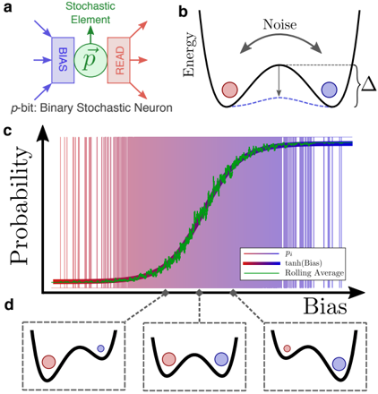
The image illustrates the concept of a binary stochastic neuron (p-bit) and its behavior in terms of energy landscapes and probability distributions. It consists of four sub-figures: a schematic of the neuron (a), an energy landscape representation (b), a probability vs. bias plot (c), and three energy landscape examples corresponding to different bias levels (d).
### Components/Axes
**Sub-figure a:**
* **Elements:**
* "BIAS" (blue rectangle): Input to the stochastic element.
* "Stochastic Element" (green circle with "p" inside and an arrow): Represents the core stochastic processing unit.
* "READ" (red rectangle): Output of the neuron.
* **Arrows:** Indicate the flow of information.
* **Label:** "p-bit: Binary Stochastic Neuron" - Describes the overall system.
**Sub-figure b:**
* **Axes:**
* Vertical axis: "Energy"
* **Curve:** A double-well potential energy landscape.
* **Elements:**
* Red and blue circles: Represent the two possible states of the p-bit.
* "Noise" (gray double-headed arrow): Indicates the influence of noise on the system.
* "Δ" (black bracket with label): Represents the energy barrier between the two states.
* Dashed blue line: Represents the energy level of the lower well.
**Sub-figure c:**
* **Axes:**
* Vertical axis: "Probability" (ranging from approximately 0 to 1).
* Horizontal axis: "Bias"
* **Data Series:**
* Red vertical lines: Represent individual samples of the p-bit output.
* Blue line: "tanh(Bias)" - Represents the theoretical probability based on the hyperbolic tangent function of the bias. It is approximately 0 for low bias values and 1 for high bias values.
* Green line: "Rolling Average" - Represents the smoothed probability based on a rolling average of the p-bit output. It follows a sigmoidal curve, transitioning from approximately 0 to 1 as the bias increases.
* **Background:** Gradient from red on the left to blue on the right, visually representing the influence of bias.
* **Legend:** Located in the middle-right of the chart.
**Sub-figure d:**
* Three separate diagrams, each showing a double-well potential energy landscape similar to sub-figure b.
* Each diagram has a red and blue circle representing the two possible states.
* The relative depths of the two wells vary, representing different bias levels.
### Detailed Analysis
**Sub-figure a:**
* The diagram shows a simplified model of a stochastic neuron. The bias input influences the stochastic element, which then produces an output that can be read.
**Sub-figure b:**
* The energy landscape illustrates the two possible states of the p-bit as residing in the two wells. The "Noise" allows the p-bit to transition between these states. The energy barrier "Δ" determines the difficulty of switching states.
**Sub-figure c:**
* **Red Vertical Lines:** These lines are dense on the left side of the chart, indicating a high probability of being in the "red" state (approximately 0 probability). On the right side, the lines are dense, indicating a high probability of being in the "blue" state (approximately 1 probability).
* **Blue Line (tanh(Bias)):** This line starts at approximately 0 for low bias values and gradually increases to approximately 1 for high bias values.
* **Green Line (Rolling Average):** This line closely follows the trend of the blue line but is smoother due to the averaging effect. It starts at approximately 0 and increases to approximately 1 as the bias increases.
* The three gray diamonds on the x-axis of the plot in (c) correspond to the three energy landscapes shown in (d).
**Sub-figure d:**
* The left diagram shows a landscape where the red state has a lower energy than the blue state, corresponding to a low bias.
* The middle diagram shows a landscape where the two states have approximately equal energy, corresponding to an intermediate bias.
* The right diagram shows a landscape where the blue state has a lower energy than the red state, corresponding to a high bias.
### Key Observations
* The probability of the p-bit being in a particular state is directly related to the energy landscape and the applied bias.
* The rolling average provides a smoothed representation of the p-bit's behavior, filtering out some of the noise.
* The tanh(Bias) function provides a theoretical model for the probability, which is closely approximated by the rolling average.
### Interpretation
The image demonstrates how a binary stochastic neuron operates. The bias input shifts the energy landscape, influencing the probability of the neuron being in one of two states. Noise allows the neuron to transition between these states, and the rolling average provides a stable estimate of the probability. The tanh(Bias) function provides a mathematical model for this behavior. The energy landscape diagrams in (d) visually represent how the bias affects the relative stability of the two states. This type of neuron can be used in various applications, such as probabilistic computing and neural networks.