## Diagram: Binary Stochastic Neuron Model and Energy Landscape Analysis
### Overview
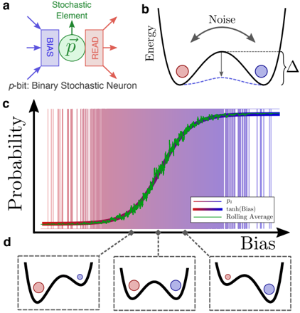
The image presents a technical diagram of a binary stochastic neuron model (a), its energy landscape (b), a probability curve (c), and bias-dependent energy state visualizations (d). The components illustrate how stochastic neurons process inputs, manage noise, and convert bias into probabilistic outputs.
### Components/Axes
**a. Binary Stochastic Neuron Diagram**
- **Components**:
- **p-bit**: Binary stochastic neuron (blue box)
- **Stochastic Element**: Green circle labeled "Stochastic Element"
- **READ**: Red box labeled "READ"
- **Flow**: Arrows indicate input (p-bit → Stochastic Element) and output (Stochastic Element → READ).
- **Labels**:
- "p-bit: Binary Stochastic Neuron" (top-left)
- "Stochastic Element" (green)
- "READ" (red)
**b. Energy Landscape**
- **Axes**: Energy (y-axis, implicit) vs. Position (x-axis, implicit).
- **Elements**:
- Parabolic energy well with two states:
- **Red dot**: High-energy state (unstable)
- **Blue dot**: Low-energy state (stable)
- **Noise**: Curved arrow labeled "Noise" between states.
- **Δ**: Energy difference between states (vertical arrow).
**c. Probability vs. Bias Graph**
- **Axes**:
- **y-axis**: Probability (labeled "Probability")
- **x-axis**: Bias (labeled "Bias")
- **Data Series**:
- **Pi (red line)**: Probability of firing (P_i)
- **tanh(Bias) (purple line)**: Sigmoid function of bias
- **Rolling Average (green line)**: Smoothed version of Pi
- **Legend**: Located at bottom-right, with color-coded labels.
**d. Bias-Dependent Energy States**
- **Insets**: Three energy landscapes (left to right) showing increasing bias.
- **Red dot**: High-energy state (unstable)
- **Blue dot**: Low-energy state (stable)
- **Δ**: Energy difference increases with bias (larger Δ in rightmost inset).
### Detailed Analysis
**c. Probability vs. Bias Graph Trends**
1. **Pi (red line)**:
- Starts near 0 at low bias, increases linearly with bias.
- Reaches ~0.8 probability at high bias.
2. **tanh(Bias) (purple line)**:
- Sigmoid curve: ~0.1 at low bias, ~0.9 at high bias.
3. **Rolling Average (green line)**:
- Smooths Pi's fluctuations, closely follows tanh(Bias) trend.
**d. Energy State Visualizations**
- As bias increases:
- Energy difference (Δ) grows (larger gap between red and blue dots).
- Red dot (high-energy state) becomes less probable, blue dot (low-energy) more probable.
### Key Observations
1. **Noise Impact**: Noise (b) causes energy state transitions, modeled as stochastic switching.
2. **Bias-Driven Probability**: Higher bias (c, d) increases the likelihood of the neuron firing (Pi → tanh(Bias)).
3. **Smoothing Effect**: Rolling Average (green) reduces noise in Pi's probability curve.
### Interpretation
The model demonstrates how stochastic neurons balance noise and bias to produce probabilistic outputs. The energy landscape (b, d) shows that bias shifts the system toward the low-energy (firing) state, while noise introduces randomness. The graph (c) quantifies this:
- **tanh(Bias)** acts as a threshold function, converting bias into a sigmoidal probability.
- **Pi** represents the raw stochastic output, smoothed by the Rolling Average to mimic real-world neural behavior.
- The energy difference (Δ) in d directly correlates with the neuron's sensitivity to bias, explaining how external inputs modulate firing probability.
This framework aligns with biophysical neuron models, where stochastic elements and energy landscapes explain decision-making under uncertainty.