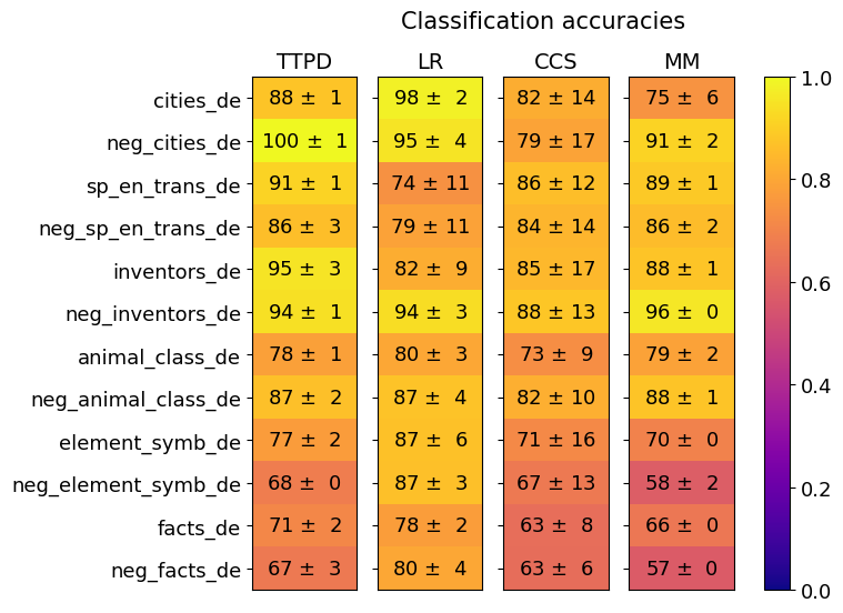
## Heatmap: Classification Accuracies ### Overview The image is a heatmap displaying the classification accuracies of four different models (TTPD, LR, CCS, and MM) across various German language datasets. The color intensity represents the accuracy score, ranging from dark blue (0.0) to bright yellow (1.0). Each cell contains the accuracy score and its associated uncertainty (± value). ### Components/Axes * **Title:** Classification accuracies * **Columns (Models):** TTPD, LR, CCS, MM * **Rows (Datasets):** cities\_de, neg\_cities\_de, sp\_en\_trans\_de, neg\_sp\_en\_trans\_de, inventors\_de, neg\_inventors\_de, animal\_class\_de, neg\_animal\_class\_de, element\_symb\_de, neg\_element\_symb\_de, facts\_de, neg\_facts\_de * **Colorbar:** Ranges from 0.0 (dark blue) to 1.0 (bright yellow), representing the classification accuracy score. ### Detailed Analysis Here's a breakdown of the accuracy scores for each model and dataset: * **cities\_de:** * TTPD: 88 ± 1 * LR: 98 ± 2 * CCS: 82 ± 14 * MM: 75 ± 6 * **neg\_cities\_de:** * TTPD: 100 ± 1 * LR: 95 ± 4 * CCS: 79 ± 17 * MM: 91 ± 2 * **sp\_en\_trans\_de:** * TTPD: 91 ± 1 * LR: 74 ± 11 * CCS: 86 ± 12 * MM: 89 ± 1 * **neg\_sp\_en\_trans\_de:** * TTPD: 86 ± 3 * LR: 79 ± 11 * CCS: 84 ± 14 * MM: 86 ± 2 * **inventors\_de:** * TTPD: 95 ± 3 * LR: 82 ± 9 * CCS: 85 ± 17 * MM: 88 ± 1 * **neg\_inventors\_de:** * TTPD: 94 ± 1 * LR: 94 ± 3 * CCS: 88 ± 13 * MM: 96 ± 0 * **animal\_class\_de:** * TTPD: 78 ± 1 * LR: 80 ± 3 * CCS: 73 ± 9 * MM: 79 ± 2 * **neg\_animal\_class\_de:** * TTPD: 87 ± 2 * LR: 87 ± 4 * CCS: 82 ± 10 * MM: 88 ± 1 * **element\_symb\_de:** * TTPD: 77 ± 2 * LR: 87 ± 6 * CCS: 71 ± 16 * MM: 70 ± 0 * **neg\_element\_symb\_de:** * TTPD: 68 ± 0 * LR: 87 ± 3 * CCS: 67 ± 13 * MM: 58 ± 2 * **facts\_de:** * TTPD: 71 ± 2 * LR: 78 ± 2 * CCS: 63 ± 8 * MM: 66 ± 0 * **neg\_facts\_de:** * TTPD: 67 ± 3 * LR: 80 ± 4 * CCS: 63 ± 6 * MM: 57 ± 0 ### Key Observations * LR generally performs well across all datasets, often achieving high accuracy scores. * CCS has the highest uncertainty (± values) in its accuracy scores compared to other models. * TTPD shows high accuracy on "neg\_cities\_de" (100 ± 1). * MM shows the lowest accuracy on "neg\_facts\_de" (57 ± 0). ### Interpretation The heatmap provides a visual comparison of the classification performance of four different models on a range of German language datasets. The color-coding allows for quick identification of the best-performing models for each dataset. The uncertainty values provide insight into the stability and reliability of each model's performance. The data suggests that LR is a robust model, while CCS may be more sensitive to the specific dataset. The "neg\_" prefixed datasets likely represent negative examples or counterfactuals, and the varying performance across these datasets highlights the models' ability to handle such cases.

## Heatmap: Classification Accuracies ### Overview This image presents a heatmap displaying classification accuracies for various datasets and models. The heatmap uses a color gradient to represent accuracy values, ranging from 0.0 (dark blue) to 1.0 (bright yellow). The data is organized in a table format, with datasets listed on the y-axis and models on the x-axis. Each cell in the heatmap represents the accuracy of a specific model on a specific dataset, along with a standard deviation. ### Components/Axes * **Y-axis (Datasets):** * cities\_de * neg\_cities\_de * sp\_en\_trans\_de * neg\_sp\_en\_trans\_de * inventors\_de * neg\_inventors\_de * animal\_class\_de * neg\_animal\_class\_de * element\_symb\_de * neg\_element\_symb\_de * facts\_de * neg\_facts\_de * **X-axis (Models):** * TTPD * LR * CCS * MM * **Color Scale (Legend):** Located on the right side of the heatmap, ranging from 0.0 (dark blue) to 1.0 (bright yellow). * **Title:** "Classification accuracies" positioned at the top-center of the heatmap. ### Detailed Analysis The heatmap displays accuracy values in the format "Mean ± Standard Deviation". I will analyze each row (dataset) and column (model) to extract the data. * **cities\_de:** * TTPD: 88 ± 1 * LR: 98 ± 2 * CCS: 82 ± 14 * MM: 75 ± 6 * **neg\_cities\_de:** * TTPD: 100 ± 1 * LR: 95 ± 4 * CCS: 79 ± 17 * MM: 91 ± 2 * **sp\_en\_trans\_de:** * TTPD: 91 ± 1 * LR: 74 ± 11 * CCS: 86 ± 12 * MM: 89 ± 1 * **neg\_sp\_en\_trans\_de:** * TTPD: 86 ± 3 * LR: 79 ± 11 * CCS: 84 ± 14 * MM: 86 ± 2 * **inventors\_de:** * TTPD: 95 ± 3 * LR: 82 ± 9 * CCS: 85 ± 17 * MM: 88 ± 1 * **neg\_inventors\_de:** * TTPD: 94 ± 1 * LR: 94 ± 3 * CCS: 88 ± 13 * MM: 96 ± 0 * **animal\_class\_de:** * TTPD: 78 ± 1 * LR: 80 ± 3 * CCS: 73 ± 9 * MM: 79 ± 2 * **neg\_animal\_class\_de:** * TTPD: 87 ± 2 * LR: 87 ± 4 * CCS: 82 ± 10 * MM: 88 ± 1 * **element\_symb\_de:** * TTPD: 77 ± 2 * LR: 87 ± 6 * CCS: 71 ± 16 * MM: 70 ± 0 * **neg\_element\_symb\_de:** * TTPD: 68 ± 0 * LR: 87 ± 3 * CCS: 67 ± 13 * MM: 58 ± 2 * **facts\_de:** * TTPD: 71 ± 2 * LR: 78 ± 2 * CCS: 63 ± 8 * MM: 66 ± 0 * **neg\_facts\_de:** * TTPD: 67 ± 3 * LR: 80 ± 4 * CCS: 63 ± 6 * MM: 57 ± 0 ### Key Observations * **LR consistently performs well:** The LR model generally achieves high accuracy across most datasets, often exceeding 90%. * **TTPD shows variability:** TTPD's performance varies significantly depending on the dataset. It performs exceptionally well on 'neg\_cities\_de' (100 ± 1) but lower on 'neg\_element\_symb\_de' (68 ± 0). * **CCS and MM generally lower accuracy:** CCS and MM models tend to have lower accuracy scores compared to LR and, in some cases, TTPD. * **Negative datasets:** The "neg\_" prefixed datasets generally have slightly different accuracy profiles compared to their non-negative counterparts. * **Low accuracy for MM on several datasets:** MM consistently shows the lowest accuracy for 'element\_symb\_de', 'neg\_element\_symb\_de', 'facts\_de', and 'neg\_facts\_de', often around 57-70%. ### Interpretation This heatmap provides a comparative analysis of the performance of four classification models (TTPD, LR, CCS, and MM) on twelve different datasets, all seemingly in the German language ("\_de" suffix). The "neg\_" datasets likely represent negative examples or adversarial data. The consistently high performance of the LR model suggests it is a robust classifier for these datasets. The variability in TTPD's performance indicates it may be more sensitive to the specific characteristics of each dataset. The lower accuracy of CCS and MM suggests they may be less effective for these particular classification tasks. The differences in accuracy between the original and negative datasets highlight the importance of considering adversarial examples when evaluating model performance. The low accuracy of MM on certain datasets could indicate a weakness in its ability to generalize to those specific types of data. The color gradient effectively visualizes the performance differences, allowing for quick identification of the best and worst performing models for each dataset. The inclusion of standard deviation provides a measure of the uncertainty associated with each accuracy estimate. This data could be used to select the most appropriate model for a given task or to identify areas where further model development is needed.

## Heatmap: Classification Accuracies ### Overview The image is a heatmap titled "Classification accuracies" that displays the performance (accuracy with standard deviation) of four different classification methods (TTPD, LR, CCS, MM) across twelve different datasets. The performance is encoded using a color gradient, with a corresponding color bar legend on the right side of the chart. ### Components/Axes * **Title:** "Classification accuracies" (centered at the top). * **Y-axis (Left):** Lists 12 dataset names. From top to bottom: 1. `cities_de` 2. `neg_cities_de` 3. `sp_en_trans_de` 4. `neg_sp_en_trans_de` 5. `inventors_de` 6. `neg_inventors_de` 7. `animal_class_de` 8. `neg_animal_class_de` 9. `element_symb_de` 10. `neg_element_symb_de` 11. `facts_de` 12. `neg_facts_de` * **X-axis (Top):** Lists 4 method names. From left to right: 1. `TTPD` 2. `LR` 3. `CCS` 4. `MM` * **Legend (Right):** A vertical color bar labeled from `0.0` (bottom, dark purple) to `1.0` (top, bright yellow). The gradient transitions from purple through red and orange to yellow, indicating increasing accuracy. * **Data Cells:** A 12x4 grid. Each cell contains a numerical value in the format `XX ± Y`, representing the mean accuracy percentage and its standard deviation. The cell's background color corresponds to the mean accuracy value according to the legend. ### Detailed Analysis Below is the extracted data for each cell, organized by dataset (row) and method (column). Values are percentages. | Dataset (Y-axis) | TTPD (Column 1) | LR (Column 2) | CCS (Column 3) | MM (Column 4) | | :--- | :--- | :--- | :--- | :--- | | **cities_de** | 88 ± 1 (Yellow) | 98 ± 2 (Bright Yellow) | 82 ± 14 (Orange) | 75 ± 6 (Orange-Red) | | **neg_cities_de** | 100 ± 1 (Bright Yellow) | 95 ± 4 (Yellow) | 79 ± 17 (Orange) | 91 ± 2 (Yellow) | | **sp_en_trans_de** | 91 ± 1 (Yellow) | 74 ± 11 (Orange) | 86 ± 12 (Orange-Yellow) | 89 ± 1 (Yellow) | | **neg_sp_en_trans_de** | 86 ± 3 (Orange-Yellow) | 79 ± 11 (Orange) | 84 ± 14 (Orange) | 86 ± 2 (Orange-Yellow) | | **inventors_de** | 95 ± 3 (Yellow) | 82 ± 9 (Orange) | 85 ± 17 (Orange) | 88 ± 1 (Yellow) | | **neg_inventors_de** | 94 ± 1 (Yellow) | 94 ± 3 (Yellow) | 88 ± 13 (Orange-Yellow) | 96 ± 0 (Bright Yellow) | | **animal_class_de** | 78 ± 1 (Orange) | 80 ± 3 (Orange) | 73 ± 9 (Orange) | 79 ± 2 (Orange) | | **neg_animal_class_de** | 87 ± 2 (Orange-Yellow) | 87 ± 4 (Orange-Yellow) | 82 ± 10 (Orange) | 88 ± 1 (Yellow) | | **element_symb_de** | 77 ± 2 (Orange) | 87 ± 6 (Orange-Yellow) | 71 ± 16 (Orange-Red) | 70 ± 0 (Orange-Red) | | **neg_element_symb_de** | 68 ± 0 (Orange-Red) | 87 ± 3 (Orange-Yellow) | 67 ± 13 (Red) | 58 ± 2 (Red-Purple) | | **facts_de** | 71 ± 2 (Orange-Red) | 78 ± 2 (Orange) | 63 ± 8 (Red) | 66 ± 0 (Red) | | **neg_facts_de** | 67 ± 3 (Red) | 80 ± 4 (Orange) | 63 ± 6 (Red) | 57 ± 0 (Red-Purple) | ### Key Observations 1. **Method Performance:** * **LR (Logistic Regression?)** shows consistently high and stable performance across most datasets, often achieving the highest or second-highest accuracy (e.g., 98±2 on `cities_de`, 94±3 on `neg_inventors_de`). Its lowest score is 74±11 on `sp_en_trans_de`. * **TTPD** also performs very well, achieving the highest score on several datasets (100±1 on `neg_cities_de`, 95±3 on `inventors_de`). It shows a significant performance drop on the last four datasets (`element_symb_de` to `neg_facts_de`). * **MM** has high variance. It excels on some datasets (96±0 on `neg_inventors_de`, 91±2 on `neg_cities_de`) but performs poorly on others, notably achieving the lowest scores in the table on `neg_element_symb_de` (58±2) and `neg_facts_de` (57±0). * **CCS** generally has the lowest average performance and the highest standard deviations (uncertainty), indicating less consistent results. Its scores are often in the 60s, 70s, or low 80s. 2. **Dataset Difficulty:** * The datasets with the `_de` suffix (likely German language tasks) appear to be more challenging for all methods. The bottom four rows (`element_symb_de`, `neg_element_symb_de`, `facts_de`, `neg_facts_de`) contain the lowest accuracy scores across the board. * The `neg_` prefixed datasets (possibly negation or adversarial examples) do not show a uniform pattern of being harder. For example, `neg_cities_de` and `neg_inventors_de` have very high accuracies, while `neg_element_symb_de` and `neg_facts_de` are among the hardest. 3. **Uncertainty (Standard Deviation):** * The standard deviations vary greatly. Some cells have very low uncertainty (e.g., `neg_inventors_de`/MM: 96 ± 0, `neg_element_symb_de`/TTPD: 68 ± 0), suggesting highly consistent results. * Others have very high uncertainty (e.g., `cities_de`/CCS: 82 ± 14, `inventors_de`/CCS: 85 ± 17), indicating the model's performance was highly variable across runs or folds for that specific task-method combination. ### Interpretation This heatmap provides a comparative analysis of four classification techniques on a suite of tasks, likely related to natural language processing or knowledge probing, given dataset names like `cities`, `inventors`, `animal_class`, and `element_symb`. The `neg_` prefix suggests tests on negated or counterfactual versions of these concepts. The data suggests that **LR is the most robust and reliable method** across this diverse set of tasks, maintaining high accuracy with relatively low variance. **TTPD is a strong performer** but shows a clear weakness on what appear to be more specialized or difficult knowledge-based tasks (elements, facts). The poor and inconsistent performance of **CCS** might indicate it is less suitable for these specific types of classification problems or requires different tuning. **MM is a high-risk, high-reward method**; it can achieve near-perfect accuracy on some tasks but fails dramatically on others, making its application less predictable. The significant performance drop for all methods on the bottom four datasets indicates these tasks (`element_symb_de`, `facts_de` and their negations) are fundamentally more difficult. This could be due to the nature of the knowledge required (scientific symbols, abstract facts), greater ambiguity, or a more challenging data distribution. The high standard deviations for CCS on many tasks further highlight its instability compared to the more consistent LR and TTPD.

## Heatmap: Classification Accuracies ### Overview The image is a heatmap comparing classification accuracies across four methods (TTPD, LR, CCS, MM) for 12 categories. Accuracy values are represented by color intensity (purple = 0.0, yellow = 1.0) and numerical values with confidence intervals (e.g., "88 ± 1"). The heatmap emphasizes performance differences between methods and categories. ### Components/Axes - **X-axis (Methods)**: TTPD, LR, CCS, MM (left to right). - **Y-axis (Categories)**: 12 rows labeled: - cities_de - neg_cities_de - sp_en_trans_de - neg_sp_en_trans_de - inventors_de - neg_inventors_de - animal_class_de - neg_animal_class_de - element_symb_de - neg_element_symb_de - facts_de - neg_facts_de - **Legend**: Color gradient from purple (0.0) to yellow (1.0), with numerical midpoint labels (0.2, 0.4, 0.6, 0.8, 1.0). Positioned on the right. ### Detailed Analysis - **TTPD Column**: - Highest accuracies overall (e.g., 100 ± 1 for neg_cities_de). - Lowest: 67 ± 3 (neg_facts_de). - **LR Column**: - Strong performance (e.g., 98 ± 2 for cities_de). - Lowest: 74 ± 11 (sp_en_trans_de). - **CCS Column**: - Moderate variability (e.g., 86 ± 12 for sp_en_trans_de). - Lowest: 63 ± 8 (facts_de). - **MM Column**: - Mixed results (e.g., 96 ± 0 for neg_inventors_de). - Lowest: 57 ± 0 (neg_facts_de). ### Key Observations 1. **TTPD Dominance**: Outperforms other methods in 8/12 categories, with 100% accuracy in neg_cities_de. 2. **CCS Variability**: Largest confidence intervals (e.g., ±17 for inventors_de), suggesting unstable results. 3. **neg_facts_de Weakness**: All methods score ≤67%, with MM at 57 ± 0 (no confidence interval). 4. **Color Consistency**: High values (e.g., 98 ± 2) align with yellow tones; low values (e.g., 58 ± 2) match purple. ### Interpretation The data suggests **TTPD** is the most reliable method, particularly for structured categories like cities and inventors. **CCS** shows inconsistent performance, possibly due to noisy data or overfitting (large confidence intervals). The **neg_facts_de** category is a notable outlier, performing poorly across all methods, indicating potential challenges in negative fact classification. The absence of confidence intervals for MM in neg_facts_de (57 ± 0) may imply deterministic results or data limitations. Overall, TTPD and LR demonstrate robustness, while CCS requires further validation for reliability.