## Diagram: Multi-Head Neural Network Architecture with Loss Functions
### Overview
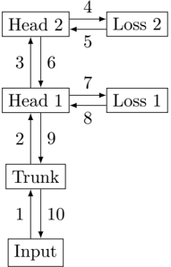
The image displays a technical block diagram illustrating the architecture of a neural network model featuring a shared trunk and two separate heads, each with its own loss function. The diagram uses rectangular boxes to represent components and numbered, directional arrows to indicate the flow of data or gradients between them. The overall flow is vertical, from the input at the bottom to the final head at the top.
### Components/Axes
The diagram consists of six primary rectangular components arranged in a vertical hierarchy with two side branches:
1. **Input**: Located at the bottom center of the diagram.
2. **Trunk**: Positioned directly above the "Input" box.
3. **Head 1**: Located above the "Trunk" box.
4. **Head 2**: Positioned at the top center, above "Head 1".
5. **Loss 1**: Placed to the right of "Head 1".
6. **Loss 2**: Placed to the right of "Head 2".
The connections between these components are represented by ten numbered, directional arrows. The numbers (1 through 10) are placed adjacent to their corresponding arrows.
### Detailed Analysis
The flow of operations, as indicated by the numbered arrows, is as follows:
* **Arrow 1**: Points upward from **Input** to **Trunk**.
* **Arrow 2**: Points upward from **Trunk** to **Head 1**.
* **Arrow 3**: Points upward from **Head 1** to **Head 2**.
* **Arrow 4**: Points rightward from **Head 2** to **Loss 2**.
* **Arrow 5**: Points leftward from **Loss 2** back to **Head 2**.
* **Arrow 6**: Points downward from **Head 2** to **Head 1**.
* **Arrow 7**: Points rightward from **Head 1** to **Loss 1**.
* **Arrow 8**: Points leftward from **Loss 1** back to **Head 1**.
* **Arrow 9**: Points downward from **Head 1** to **Trunk**.
* **Arrow 10**: Points downward from **Trunk** to **Input**.
This creates two distinct cycles:
1. A forward pass cycle: Input → Trunk → Head 1 → Head 2 → Loss 2.
2. A backward pass/gradient flow cycle: Loss 2 → Head 2 → Head 1 → Trunk → Input.
A similar, nested cycle exists for Head 1 and Loss 1: Head 1 → Loss 1 → Head 1.
### Key Observations
1. **Hierarchical Structure**: The model has a clear hierarchy: a shared **Trunk** processes the **Input**, which then feeds into two sequential heads (**Head 1** and **Head 2**).
2. **Dual-Head Design**: The architecture employs two separate output heads, suggesting a multi-task or multi-objective learning setup.
3. **Independent Loss Functions**: Each head (**Head 1**, **Head 2**) is connected to its own dedicated loss module (**Loss 1**, **Loss 2**), allowing for separate error calculation and likely separate optimization targets for each task.
4. **Bidirectional Flow**: The numbered arrows indicate bidirectional communication. The upward arrows (1, 2, 3, 4, 7) likely represent the forward propagation of data. The downward and return arrows (5, 6, 8, 9, 10) likely represent the backward propagation of gradients or error signals during training.
5. **Nested Feedback Loops**: The diagram shows that gradients from **Loss 2** flow back through **Head 2** and then into **Head 1** and the **Trunk**. Gradients from **Loss 1** flow back only into **Head 1**. This implies that **Head 1** receives gradient signals from both its own loss and the loss of the subsequent head (**Head 2**).
### Interpretation
This diagram represents a **multi-task learning neural network architecture**. The shared **Trunk** learns a common feature representation from the **Input** data. These features are then used by two separate task-specific modules, **Head 1** and **Head 2**.
The presence of two distinct loss functions (**Loss 1**, **Loss 2**) confirms that the network is being trained to perform two different tasks simultaneously. The sequential connection from **Head 1** to **Head 2** suggests a potential dependency; the task performed by **Head 2** might be more complex or higher-level, building upon the output or features from **Head 1**.
The numbered flow is critical for understanding the training dynamics. During a forward pass (arrows 1→2→3→4/7), data flows up to generate predictions and compute losses. During backpropagation (arrows 5→6→9→10 and 8), gradients flow downward to update the network's weights. The key architectural insight is that **Head 1** and the shared **Trunk** are updated by gradient signals from *both* tasks, forcing them to learn features useful for both objectives. **Head 2** is only updated by its specific task loss. This design balances shared representation learning with task-specific specialization.