## Line Chart: Gradient Variance vs. Training Epochs
### Overview
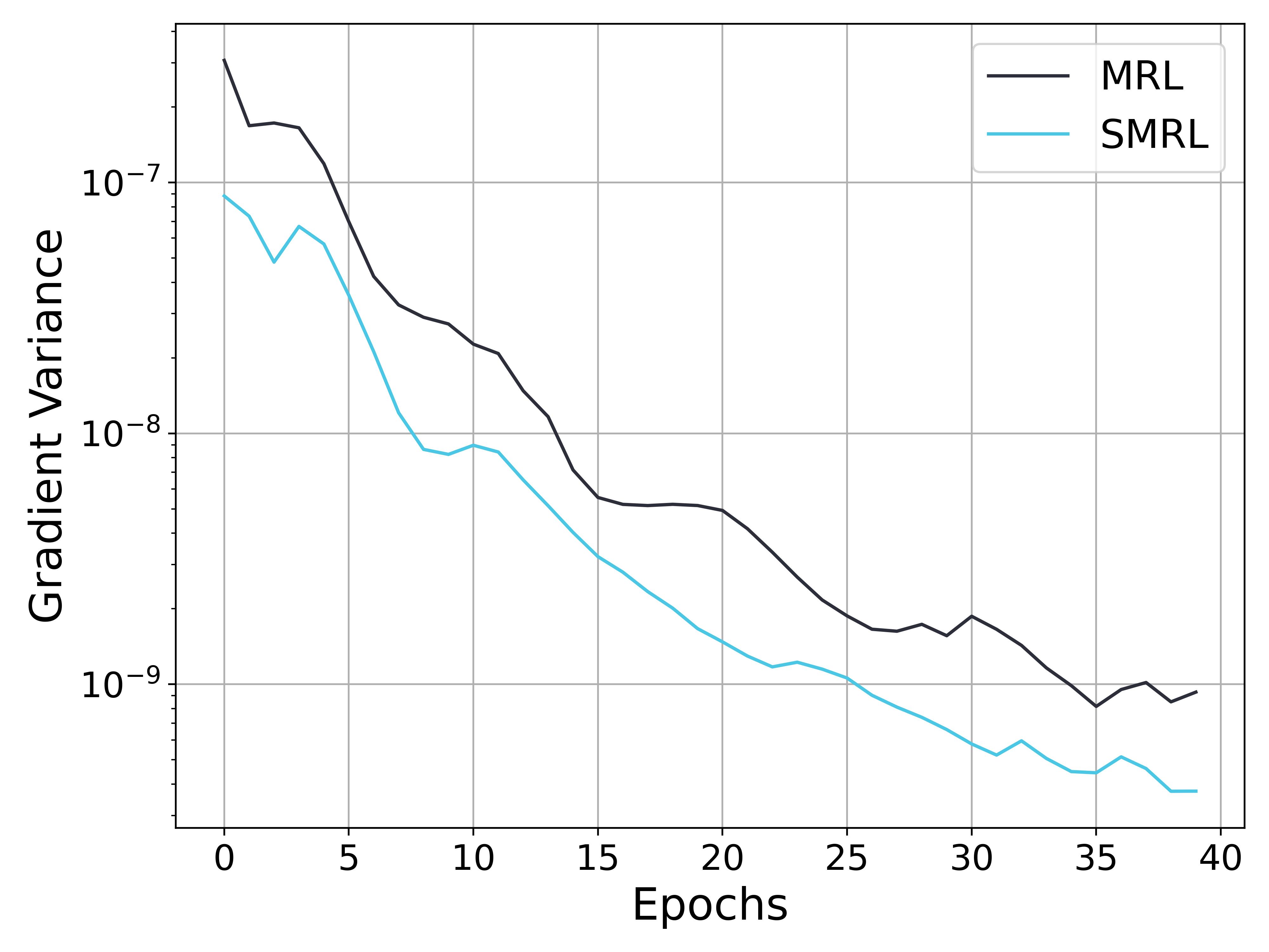
This image is a line chart comparing the "Gradient Variance" of two methods, labeled **MRL** and **SMRL**, over the course of 40 training epochs. The chart uses a logarithmic scale for the y-axis to visualize data spanning multiple orders of magnitude.
### Components/Axes
* **Chart Type:** Line chart with a logarithmic y-axis.
* **X-Axis:**
* **Label:** "Epochs"
* **Scale:** Linear, from 0 to 40.
* **Major Ticks:** 0, 5, 10, 15, 20, 25, 30, 35, 40.
* **Y-Axis:**
* **Label:** "Gradient Variance"
* **Scale:** Logarithmic (base 10).
* **Major Ticks (Labels):** 10⁻⁹, 10⁻⁸, 10⁻⁷.
* **Minor Ticks:** Visible between major ticks, indicating intermediate values (e.g., 2x10⁻⁹, 5x10⁻⁹).
* **Legend:**
* **Position:** Top-right corner of the plot area.
* **Items:**
1. **MRL:** Represented by a dark gray/black solid line.
2. **SMRL:** Represented by a cyan/light blue solid line.
* **Grid:** A light gray grid is present, aligned with the major ticks on both axes.
### Detailed Analysis
**Trend Verification & Data Points:**
Both data series exhibit a clear downward trend, indicating that gradient variance decreases as training progresses (epochs increase). The y-axis is logarithmic, so a straight line would indicate exponential decay.
1. **MRL (Dark Gray Line):**
* **Trend:** Starts at the highest point on the chart and follows a generally decreasing, slightly jagged path. The rate of decrease is steepest in the first ~15 epochs and becomes more gradual thereafter.
* **Approximate Key Points:**
* Epoch 0: ~4 x 10⁻⁷ (Highest point)
* Epoch 5: ~1 x 10⁻⁷
* Epoch 10: ~3 x 10⁻⁸
* Epoch 15: ~6 x 10⁻⁹
* Epoch 20: ~5 x 10⁻⁹
* Epoch 30: ~2 x 10⁻⁹ (with a small local peak)
* Epoch 40: ~1 x 10⁻⁹
2. **SMRL (Cyan Line):**
* **Trend:** Also starts high but consistently remains below the MRL line. It shows a steeper initial decline than MRL and maintains a lower variance throughout. The line has more visible small fluctuations (e.g., around epochs 3, 10, 32).
* **Approximate Key Points:**
* Epoch 0: ~9 x 10⁻⁸
* Epoch 5: ~4 x 10⁻⁸
* Epoch 10: ~9 x 10⁻⁹
* Epoch 15: ~3 x 10⁻⁹
* Epoch 20: ~1.5 x 10⁻⁹
* Epoch 30: ~6 x 10⁻¹⁰
* Epoch 40: ~3 x 10⁻¹⁰ (Lowest point on the chart)
**Spatial Grounding:** The legend is positioned in the top-right, clearly associating the dark gray line with "MRL" and the cyan line with "SMRL." The SMRL line is visually below the MRL line for the entire duration shown.
### Key Observations
1. **Consistent Performance Gap:** The SMRL method demonstrates consistently lower gradient variance than the MRL method at every epoch from 0 to 40.
2. **Convergence Behavior:** Both methods show a reduction in gradient variance over time, which is typical of a converging training process. The variance for both appears to plateau or decrease very slowly after approximately epoch 25.
3. **Relative Magnitude:** By epoch 40, the gradient variance for SMRL (~3x10⁻¹⁰) is approximately one-third to one-fourth that of MRL (~1x10⁻⁹).
4. **Volatility:** The SMRL line exhibits slightly more short-term volatility (small peaks and valleys) compared to the somewhat smoother descent of the MRL line, particularly in the later epochs.
### Interpretation
This chart provides a technical comparison of training stability between two methods, likely in the context of machine learning or optimization. Gradient variance is a metric often associated with the noise in gradient estimates during stochastic optimization; lower variance generally implies more stable and reliable updates.
* **What the data suggests:** The SMRL method appears to achieve significantly more stable training dynamics (lower gradient noise) than the MRL method. The faster initial drop in variance for SMRL might indicate quicker adaptation or more effective variance reduction in the early training phase.
* **How elements relate:** The x-axis (Epochs) represents training time/progress, while the y-axis (Gradient Variance) is a measure of optimization stability. The inverse relationship shown (variance decreases as epochs increases) is the expected behavior for a well-behaved training process. The separation between the two lines quantifies the performance difference between the MRL and SMRL algorithms.
* **Notable implications:** If gradient variance is a critical metric for the application (e.g., in reinforcement learning or fine-tuning large models), SMRL demonstrates a clear advantage. The persistent gap suggests the improvement is not transient but sustained throughout training. The chart does not show the final model performance (e.g., accuracy, reward), so while SMRL has more stable gradients, one cannot conclude from this chart alone that it results in a better final model—only that its optimization process is less noisy.