\n
## Contour Plot: Dimensionality Reduction of Text Data
### Overview
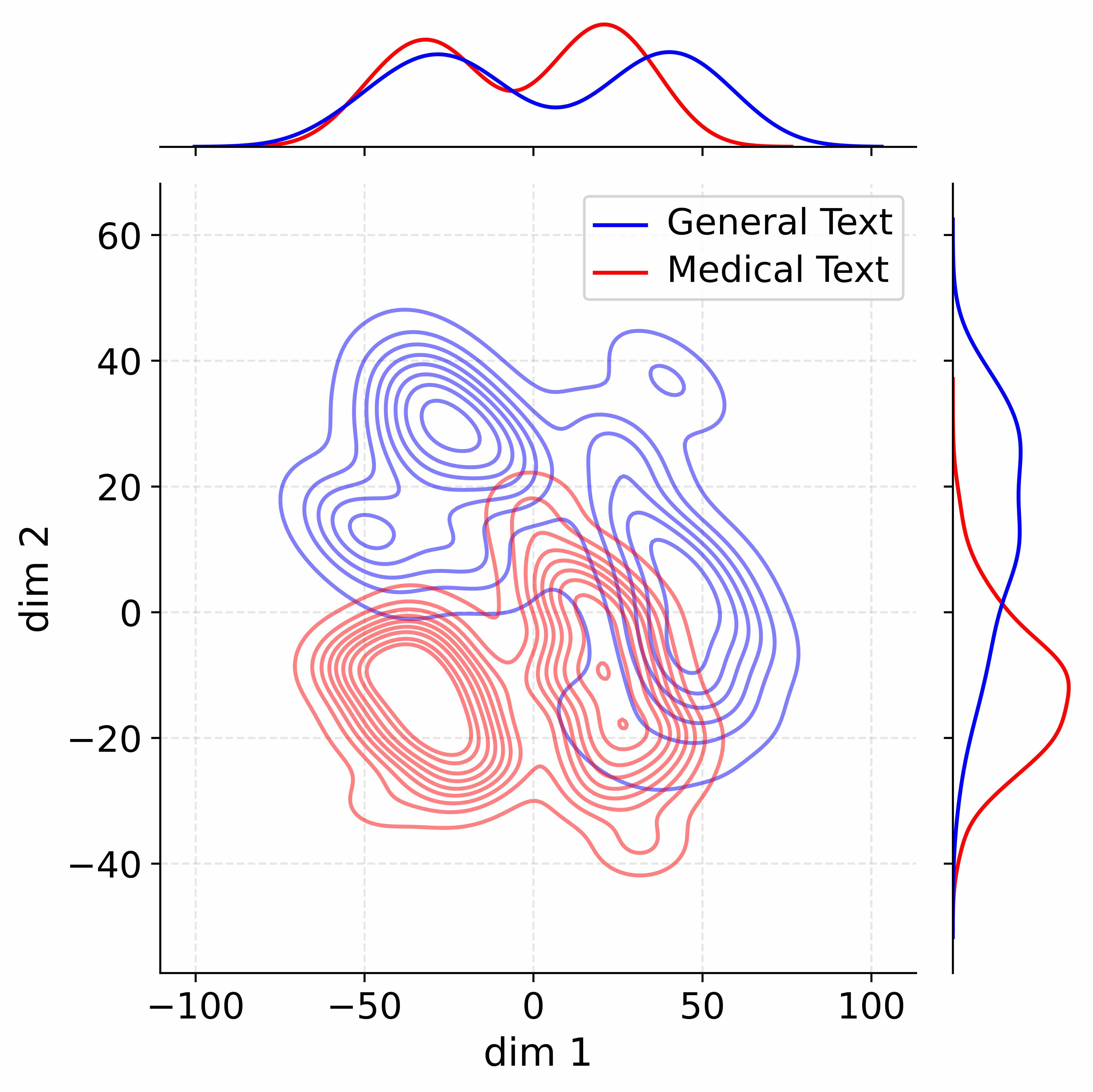
The image presents a 2D contour plot visualizing the distribution of text data reduced to two dimensions (dim 1 and dim 2). Two marginal histograms are included, one for "General Text" (blue) and one for "Medical Text" (red), showing the distribution of values along dim 1. The contour lines represent density levels, indicating areas where data points are concentrated.
### Components/Axes
* **X-axis:** "dim 1" ranging from approximately -100 to 100.
* **Y-axis:** "dim 2" ranging from approximately -50 to 60.
* **Contour Lines:** Represent density of data points. Blue contours represent "General Text", and red contours represent "Medical Text".
* **Legend:** Located in the top-right corner, associating blue with "General Text" and red with "Medical Text".
* **Marginal Histograms:** Placed along the top edge of the plot, showing the distribution of data along dim 1 for each text type. The x-axis of the histograms is "dim 1", and the y-axis represents frequency or density.
### Detailed Analysis
The contour plot shows a clear separation between the distributions of "General Text" and "Medical Text".
* **General Text (Blue):** The blue contours are concentrated in the upper-left quadrant, extending from approximately dim 1 = -75 to dim 1 = 50, and dim 2 = 0 to dim 2 = 60. The density appears highest around dim 1 = 0 and dim 2 = 40.
* **Medical Text (Red):** The red contours are primarily located in the lower-right quadrant, spanning from approximately dim 1 = -50 to dim 1 = 50, and dim 2 = -40 to dim 2 = 20. The highest density appears around dim 1 = 0 and dim 2 = -20. There is some overlap between the red and blue contours near dim 1 = 0.
**Marginal Histograms:**
* **General Text (Blue):** The histogram shows a peak around dim 1 = 50, with a long tail extending towards negative values. The histogram starts at approximately 0 frequency at dim 1 = -100, rises to a peak around dim 1 = 50 (approximately 0.8 frequency), and then declines to approximately 0.2 frequency at dim 1 = 100.
* **Medical Text (Red):** The histogram is more symmetrical and centered around dim 1 = 0. It starts at approximately 0.2 frequency at dim 1 = -100, reaches a peak around dim 1 = 0 (approximately 0.6 frequency), and declines to approximately 0.2 frequency at dim 1 = 100.
### Key Observations
* The two text types exhibit distinct distributions in the reduced dimensional space.
* There is some overlap in the distributions, suggesting that some features are shared between the two text types.
* The marginal histograms reveal differences in the distribution of dim 1 values for the two text types. General text tends to have higher values of dim 1, while medical text is more centered around 0.
* The contour lines indicate that the separation between the two text types is more pronounced in the dim 2 direction.
### Interpretation
This plot likely represents the results of a dimensionality reduction technique (e.g., PCA, t-SNE) applied to text data. The goal is to visualize high-dimensional text data in a lower-dimensional space while preserving the relationships between data points.
The clear separation between "General Text" and "Medical Text" suggests that these two types of text have different underlying characteristics that are captured by the reduced dimensions. Dim 1 appears to be a key discriminator, with general text having higher values and medical text being centered around zero. Dim 2 contributes to the separation as well, with general text tending to have higher values.
The overlap between the distributions indicates that there is some similarity between the two text types, which is expected. The marginal histograms provide additional insights into the distribution of values along dim 1 for each text type.
This visualization could be used to identify features that are important for distinguishing between general and medical text, or to explore the relationships between different types of text data. The plot suggests that the dimensionality reduction technique has successfully captured some of the key differences between these two text types.