## Chart: Training Loss Comparison and Distribution Probabilities
### Overview
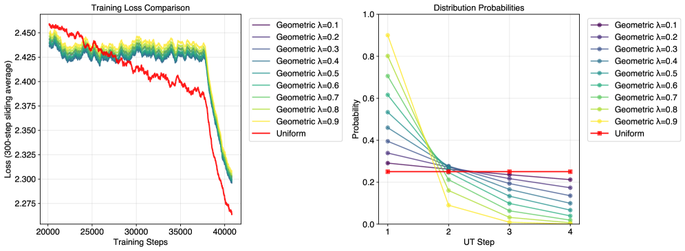
The image presents two charts side-by-side. The left chart compares the training loss of different geometric distributions against a uniform distribution. The right chart shows the distribution probabilities for each geometric distribution and the uniform distribution across four UT Steps.
### Components/Axes
**Left Chart: Training Loss Comparison**
* **Title:** Training Loss Comparison
* **X-axis:** Training Steps, ranging from 20000 to 40000 in increments of 5000.
* **Y-axis:** Loss (300-step sliding average), ranging from 2.275 to 2.450 in increments of 0.025.
* **Legend (Top-Right):**
* Purple: Geometric λ=0.1
* Dark Blue: Geometric λ=0.2
* Blue: Geometric λ=0.3
* Teal: Geometric λ=0.4
* Green-Teal: Geometric λ=0.5
* Green: Geometric λ=0.6
* Light Green: Geometric λ=0.7
* Yellow-Green: Geometric λ=0.8
* Yellow: Geometric λ=0.9
* Red: Uniform
**Right Chart: Distribution Probabilities**
* **Title:** Distribution Probabilities
* **X-axis:** UT Step, ranging from 1 to 4 in increments of 1.
* **Y-axis:** Probability, ranging from 0.0 to 1.0 in increments of 0.2.
* **Legend (Top-Right):** Same as the left chart.
* Purple: Geometric λ=0.1
* Dark Blue: Geometric λ=0.2
* Blue: Geometric λ=0.3
* Teal: Geometric λ=0.4
* Green-Teal: Geometric λ=0.5
* Green: Geometric λ=0.6
* Light Green: Geometric λ=0.7
* Yellow-Green: Geometric λ=0.8
* Yellow: Geometric λ=0.9
* Red: Uniform
### Detailed Analysis
**Left Chart: Training Loss Comparison**
* **Geometric λ=0.1 to λ=0.9:** The lines representing geometric distributions (λ=0.1 to λ=0.9) start at approximately the same loss value of 2.450 at 20000 training steps. They fluctuate slightly before generally decreasing to approximately 2.300 by 40000 training steps.
* **Uniform:** The uniform distribution starts at approximately 2.450 at 20000 training steps. It decreases more rapidly than the geometric distributions, reaching approximately 2.225 by 40000 training steps.
**Right Chart: Distribution Probabilities**
* **Geometric Distributions (λ=0.1 to λ=0.9):**
* All geometric distributions start with varying probabilities at UT Step 1 and decrease as the UT Step increases.
* Geometric λ=0.1 (Purple): Starts at approximately 0.35 and decreases to approximately 0.25 by UT Step 4.
* Geometric λ=0.2 (Dark Blue): Starts at approximately 0.50 and decreases to approximately 0.25 by UT Step 4.
* Geometric λ=0.3 (Blue): Starts at approximately 0.60 and decreases to approximately 0.25 by UT Step 4.
* Geometric λ=0.4 (Teal): Starts at approximately 0.68 and decreases to approximately 0.25 by UT Step 4.
* Geometric λ=0.5 (Green-Teal): Starts at approximately 0.75 and decreases to approximately 0.25 by UT Step 4.
* Geometric λ=0.6 (Green): Starts at approximately 0.80 and decreases to approximately 0.25 by UT Step 4.
* Geometric λ=0.7 (Light Green): Starts at approximately 0.85 and decreases to approximately 0.25 by UT Step 4.
* Geometric λ=0.8 (Yellow-Green): Starts at approximately 0.90 and decreases to approximately 0.25 by UT Step 4.
* Geometric λ=0.9 (Yellow): Starts at approximately 0.95 and decreases to approximately 0.25 by UT Step 4.
* **Uniform:** The uniform distribution (Red) maintains a constant probability of approximately 0.25 across all UT Steps.
### Key Observations
* In the Training Loss Comparison, the uniform distribution consistently achieves a lower loss than the geometric distributions as training progresses.
* In the Distribution Probabilities, the geometric distributions have higher initial probabilities that decrease with each UT Step, while the uniform distribution maintains a constant probability.
* All geometric distributions converge to a similar probability value (approximately 0.25) by UT Step 4.
### Interpretation
The charts suggest that, in this specific training scenario, the uniform distribution leads to a lower training loss compared to the geometric distributions. The distribution probabilities indicate that the geometric distributions initially favor earlier UT Steps but become more uniform-like as the UT Step increases. The uniform distribution, with its constant probability across all UT Steps, appears to be a more effective strategy for minimizing training loss in this case. The convergence of geometric distributions to a similar probability at higher UT Steps suggests that the impact of the initial distribution diminishes over time.