## Mathematical Diagram: Commutative Diagram in Equivariant K-Theory
### Overview
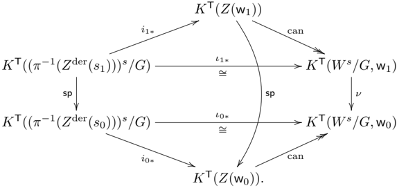
This image is a complex commutative diagram from a mathematical text, likely in the field of algebraic geometry or K-theory. It illustrates the relationships between various equivariant K-groups ($K^T$) through a series of morphisms (arrows). The diagram is composed of a central square and two triangles attached to the left side of the square, all of which are commutative.
### Components
The diagram consists of six nodes, each representing a mathematical object (a K-group), and several directed edges representing morphisms between them.
#### Nodes (Mathematical Objects)
The nodes are arranged in three columns.
* **Left Column:**
* Top-left: $K^T((\pi^{-1}(Z^{\text{der}}(s_1)))^s/G)$
* Bottom-left: $K^T((\pi^{-1}(Z^{\text{der}}(s_0)))^s/G)$
* **Center Column:**
* Top-center: $K^T(Z(w_1))$
* Bottom-center: $K^T(Z(w_0))$
* **Right Column:**
* Top-right: $K^T(W^s/G, w_1)$
* Bottom-right: $K^T(W^s/G, w_0)$
#### Edges (Morphisms)
The edges are labeled arrows indicating maps between the K-groups.
* **Horizontal Maps (Isomorphisms):**
* Top horizontal: From $K^T((\pi^{-1}(Z^{\text{der}}(s_1)))^s/G)$ to $K^T(W^s/G, w_1)$. Labeled $\iota_{1*}$. Below the arrow is the symbol $\cong$, indicating this map is an isomorphism.
* Bottom horizontal: From $K^T((\pi^{-1}(Z^{\text{der}}(s_0)))^s/G)$ to $K^T(W^s/G, w_0)$. Labeled $\iota_{0*}$. Below the arrow is the symbol $\cong$, indicating this map is an isomorphism.
* **Vertical Maps:**
* Left vertical: From $K^T((\pi^{-1}(Z^{\text{der}}(s_1)))^s/G)$ to $K^T((\pi^{-1}(Z^{\text{der}}(s_0)))^s/G)$. Labeled `sp`.
* Right vertical: From $K^T(W^s/G, w_1)$ to $K^T(W^s/G, w_0)$. Labeled $\nu$.
* Center curved vertical: From $K^T(Z(w_1))$ to $K^T(Z(w_0))$. Labeled `sp`.
* **Diagonal Maps (Top Triangle):**
* From $K^T((\pi^{-1}(Z^{\text{der}}(s_1)))^s/G)$ to $K^T(Z(w_1))$. Labeled $i_{1*}$.
* From $K^T(Z(w_1))$ to $K^T(W^s/G, w_1)$. Labeled `can`.
* **Diagonal Maps (Bottom Triangle):**
* From $K^T((\pi^{-1}(Z^{\text{der}}(s_0)))^s/G)$ to $K^T(Z(w_0))$. Labeled $i_{0*}$.
* From $K^T(Z(w_0))$ to $K^T(W^s/G, w_0)$. Labeled `can`.
### Diagram Structure and Flow
The diagram is structured to show the commutativity of several paths.
1. **Central Square:** The square formed by the four corner nodes and the horizontal and vertical arrows between them is commutative. This means the composition of maps along the top and right ($\nu \circ \iota_{1*}$) is equal to the composition along the left and bottom ($\iota_{0*} \circ \text{sp}$).
$$ \nu \circ \iota_{1*} = \iota_{0*} \circ \text{sp} $$
2. **Top Triangle:** The triangle formed by the top-left, top-center, and top-right nodes is commutative. The horizontal map $\iota_{1*}$ is the composition of the two diagonal maps.
$$ \iota_{1*} = \text{can} \circ i_{1*} $$
3. **Bottom Triangle:** Similarly, the bottom triangle is commutative. The horizontal map $\iota_{0*}$ is the composition of the two diagonal maps.
$$ \iota_{0*} = \text{can} \circ i_{0*} $$
4. **Overall Commutativity:** The entire diagram is commutative. For example, the path from the top-left node to the bottom-right node is the same regardless of the route taken.
* Path 1: $K^T((\pi^{-1}(Z^{\text{der}}(s_1)))^s/G) \xrightarrow{\text{sp}} K^T((\pi^{-1}(Z^{\text{der}}(s_0)))^s/G) \xrightarrow{i_{0*}} K^T(Z(w_0)) \xrightarrow{\text{can}} K^T(W^s/G, w_0)$
* Path 2: $K^T((\pi^{-1}(Z^{\text{der}}(s_1)))^s/G) \xrightarrow{i_{1*}} K^T(Z(w_1)) \xrightarrow{\text{sp}} K^T(Z(w_0)) \xrightarrow{\text{can}} K^T(W^s/G, w_0)$
* Path 3: $K^T((\pi^{-1}(Z^{\text{der}}(s_1)))^s/G) \xrightarrow{i_{1*}} K^T(Z(w_1)) \xrightarrow{\text{can}} K^T(W^s/G, w_1) \xrightarrow{\nu} K^T(W^s/G, w_0)$
### Interpretation
This diagram likely illustrates a compatibility condition or a change-of-base result in equivariant K-theory.
* The vertical maps labeled `sp` likely represent "specialization" maps, relating K-theory of a general fiber (associated with $s_1$ or $w_1$) to a special fiber (associated with $s_0$ or $w_0$).
* The maps labeled `can` are "canonical" maps.
* The maps $i_{1*}$ and $i_{0*}$ are pushforward maps induced by inclusions.
* The horizontal isomorphisms $\iota_{1*}$ and $\iota_{0*}$ suggest an identification between the K-groups on the left and right, possibly due to some form of homotopy invariance or localization principle.
* The commutativity of the diagram ensures that these different operations (specialization, canonical maps, pushforwards) are compatible with each other. For instance, specializing and then taking the canonical map is the same as taking the canonical map and then specializing (as seen in the right-hand part of the diagram involving $\nu$ and `sp`).