\n
## Diagram and 3D Surface Plot: Dependency Mapping and Function Visualization
### Overview
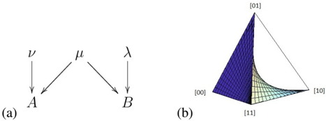
The image contains two distinct technical illustrations labeled (a) and (b). Part (a) is a directed graph or dependency diagram showing relationships between Greek letter variables and Latin letter nodes. Part (b) is a 3D surface plot rendered on a triangular or tetrahedral domain, visualizing a mathematical function or data distribution.
### Components/Axes
**Part (a) - Dependency Diagram:**
* **Nodes:** Two primary nodes labeled with uppercase Latin letters: `A` (left) and `B` (right).
* **Variables/Labels:** Three Greek letters positioned above the nodes:
* `ν` (nu) is positioned directly above node `A`.
* `μ` (mu) is positioned centrally between and above nodes `A` and `B`.
* `λ` (lambda) is positioned directly above node `B`.
* **Edges/Arrows:** Three directed arrows indicating relationships or mappings:
* An arrow points from `ν` down to `A`.
* An arrow points from `μ` down to `A`.
* An arrow points from `μ` down to `B`.
* An arrow points from `λ` down to `B`.
* **Spatial Grounding:** The diagram is laid out horizontally. `A` is on the left, `B` is on the right. The Greek letters are aligned in a row above them, with `μ` centered.
**Part (b) - 3D Surface Plot:**
* **Plot Type:** A 3D surface plot displayed within a triangular (likely 2-simplex) or tetrahedral wireframe.
* **Axes/Vertex Labels:** The vertices of the triangular base are labeled with binary pairs in square brackets:
* Bottom-left vertex: `[00]`
* Bottom-right vertex: `[10]`
* Top vertex: `[01]`
* A fourth vertex, forming the apex of the tetrahedron, is labeled `[11]`.
* **Surface:** A colored mesh surface is plotted within this domain. The surface is highest near the `[01]` vertex and curves downward towards the `[00]` and `[10]` vertices, and more steeply towards the `[11]` vertex.
* **Color Mapping:** The surface uses a color gradient. The highest region (near `[01]`) is dark blue/purple. As the surface descends, the color transitions through teal and green to a pale yellow/cream at its lowest points (near `[11]` and the edge between `[00]` and `[10]`). There is no explicit color bar or legend provided.
* **Grid:** The surface is rendered with a visible black mesh grid, emphasizing its curvature.
### Detailed Analysis
* **Part (a) Relationships:** The diagram defines a clear set of dependencies. Variables `ν` and `μ` both influence or map to node `A`. Variables `μ` and `λ` both influence or map to node `B`. Variable `μ` is the only element that has a relationship with both `A` and `B`, acting as a common factor or shared input.
* **Part (b) Surface Trend:** The visual trend of the surface is a smooth, concave descent from a single peak. The highest point is at vertex `[01]`. The surface slopes downward in all directions from this peak. The descent is most gradual towards the `[00]-[10]` edge and most precipitous towards the `[11]` vertex. The mesh grid lines follow this curvature, becoming more densely packed in areas of steeper gradient.
### Key Observations
1. **Asymmetric Dependency:** In diagram (a), the dependency is not symmetric. `A` receives inputs from two sources (`ν`, `μ`), while `B` also receives inputs from two sources (`μ`, `λ`). The shared input `μ` creates a link between the two otherwise separate chains.
2. **Function Behavior:** The surface in (b) suggests a function that is maximized at the state `[01]` and minimized at or near the state `[11]`. The smooth gradient indicates a continuous function over the domain.
3. **Domain Representation:** The use of binary pair labels (`[00]`, `[01]`, `[10]`, `[11]`) strongly suggests the plot represents a function over a space of two binary variables or a two-qubit quantum state space, where the vertices correspond to basis states. The triangular/tetrahedral shape is a common way to visualize probability distributions or functions on such a space.
### Interpretation
These two figures are likely from a technical paper in fields like quantum computing, information theory, or statistical modeling.
* **Figure (a)** is a classic graphical model or causal diagram. It could represent a probabilistic model where `A` and `B` are observed variables, and `ν`, `μ`, `λ` are latent parameters or causes. The structure suggests `μ` is a confounding variable affecting both `A` and `B`. Alternatively, in a quantum context, it could depict a circuit or gate mapping where `μ` is a two-qubit gate acting on qubits `A` and `B`.
* **Figure (b)** visualizes a key property of the system modeled in (a). Given the binary labels, it most likely plots a **fidelity, probability, or correlation measure** across the joint state space of two binary systems (e.g., two qubits). The peak at `[01]` indicates this specific state has the highest value of the measured property. The low value at `[11]` suggests an anti-correlation or a state that is suppressed by the model's dynamics. The smooth surface implies the property varies continuously as one moves between these basis states (e.g., through superposition).
**Together, the figures tell a story:** Diagram (a) defines the structure of a system with interacting components, and plot (b) quantitatively shows the outcome or behavior of that system across its entire possible state space. The notable anomaly is the specific, single-peak structure of the surface, which would be a direct consequence of the specific dependencies (especially the role of `μ`) defined in the first diagram.