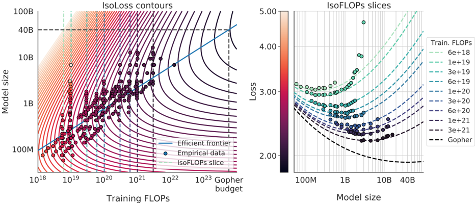
## Scatter Plots: Model Efficiency and Loss Relationships ### Overview The image contains two side-by-side scatter plots analyzing the relationship between model size, training computational resources (FLOPs), and model performance (loss). The left plot focuses on model size vs. training FLOPs with efficiency contours, while the right plot examines model size vs. loss with FLOPs-based loss contours. --- ### Components/Axes #### Left Chart (Model Size vs. Training FLOPs) - **X-axis**: Training FLOPs (log scale, 10¹⁸ to 10²³) - **Y-axis**: Model size (log scale, 100M to 100B) - **Legend**: - **Efficient frontier**: Blue solid line (optimal trade-off between model size and FLOPs) - **Empirical data**: Purple dots (observed model-FLOPs pairs) - **IsoFLOPs slice**: Dashed lines (vertical lines at specific FLOPs values: 10¹⁸, 10¹⁹, 10²⁰, 10²¹, 10²², 10²³) - **Contours**: Red-to-purple gradient lines representing IsoLoss contours (loss levels). #### Right Chart (Model Size vs. Loss) - **X-axis**: Model size (log scale, 100M to 40B) - **Y-axis**: Loss (log scale, 2.00 to 5.00) - **Legend**: - **Train. FLOPs**: Dashed lines in cyan-to-purple gradient (6e¹⁸ to 3e²¹ FLOPs) - **Gopher**: Black dashed line (baseline model) - **Color bar**: Gradient from orange (low loss) to purple (high loss), labeled 2.00–5.00. --- ### Detailed Analysis #### Left Chart - **Efficient frontier**: A straight blue line from ~10¹⁸ FLOPs (100M model) to ~10²³ FLOPs (100B model), suggesting a linear relationship between FLOPs and model size under optimal conditions. - **Empirical data**: Purple dots cluster near the efficient frontier, indicating most models operate close to this optimal trade-off. - **IsoFLOPs slices**: Vertical dashed lines at 10¹⁸, 10¹⁹, 10²⁰, 10²¹, 10²², and 10²³ FLOPs. These lines show how model size increases with FLOPs (e.g., at 10²⁰ FLOPs, model size ~1B; at 10²³ FLOPs, ~100B). - **IsoLoss contours**: Red-to-purple lines indicate that higher FLOPs allow for larger models with lower loss (e.g., 10²³ FLOPs correspond to ~100B models with loss ~2.00). #### Right Chart - **Model size vs. loss**: As model size increases, loss decreases (e.g., 100M model: loss ~4.00; 40B model: loss ~2.00). - **FLOPs-based contours**: Dashed lines show that higher FLOPs enable larger models with lower loss. For example: - 6e¹⁸ FLOPs: Model size ~100M, loss ~4.00 - 3e²⁰ FLOPs: Model size ~10B, loss ~3.00 - 1e²¹ FLOPs: Model size ~100B, loss ~2.00 - **Gopher baseline**: The black dashed line (Gopher model) shows a similar trend but with higher loss for equivalent model sizes compared to other FLOPs levels. --- ### Key Observations 1. **Efficiency trade-off**: The efficient frontier (left chart) suggests that models can scale predictably with FLOPs, but empirical data (purple dots) show variability, likely due to architectural or optimization differences. 2. **Loss reduction**: Larger models (right chart) achieve lower loss, but the rate of improvement diminishes (e.g., 10B to 100B models reduce loss from ~3.00 to ~2.00). 3. **FLOPs impact**: Higher FLOPs (left chart) enable larger models, but the right chart shows that FLOPs also directly influence loss, with higher FLOPs reducing loss more effectively. 4. **Gopher underperformance**: The Gopher baseline (right chart) lags behind other FLOPs levels, indicating it may be less optimized for the given task. --- ### Interpretation - **Efficiency vs. performance**: The left chart highlights the computational cost of scaling models, while the right chart quantifies the performance gains. Together, they suggest that increasing FLOPs improves both model size and loss, but diminishing returns occur at larger scales. - **Optimal scaling**: The efficient frontier implies that models should be designed to align with this trade-off to maximize performance per FLOP. - **Gopher’s limitations**: The Gopher baseline’s higher loss for equivalent model sizes suggests it may lack architectural innovations (e.g., sparse attention, better tokenization) to compete with FLOPs-optimized models. - **Practical implications**: For a given FLOP budget, prioritizing model size over loss may not always yield the best results—balancing both is critical. --- **Note**: All values are approximate, derived from visual inspection of the plots. Uncertainty arises from the logarithmic scales and lack of explicit numerical annotations for individual data points.