## Diagram: Commutative Diagram of Homotopy Groups ### Overview The image presents a commutative diagram illustrating relationships between homotopy groups. It shows how the homotopy group of a space (X^A, w^A) transforms into the homotopy group of another space (X, w) through different stabilization maps. ### Components/Axes * **Nodes:** * Top-left: H^T(X^A, w^A) * Top-right: H^T(X, w) * Bottom-center: H^T(X^A', w^A') * **Arrows (Maps):** * Top arrow: Stabe (from H^T(X^A, w^A) to H^T(X, w)) * Left arrow: Stab_{e/e'} (from H^T(X^A, w^A) to H^T(X^A', w^A')) * Right arrow: Stab_{e'} (from H^T(X^A', w^A') to H^T(X, w)) ### Detailed Analysis The diagram depicts a commutative relationship between different homotopy groups and stabilization maps. * **H^T(X^A, w^A):** This represents the T-equivariant homotopy group of the space X^A with a basepoint w^A. It is located at the top-left of the diagram. * **H^T(X, w):** This represents the T-equivariant homotopy group of the space X with a basepoint w. It is located at the top-right of the diagram. * **H^T(X^A', w^A'):** This represents the T-equivariant homotopy group of the space X^A' with a basepoint w^A'. It is located at the bottom-center of the diagram. * **Stab_e:** This is a stabilization map from H^T(X^A, w^A) to H^T(X, w). It is represented by the arrow going from the top-left node to the top-right node. * **Stab_{e/e'}:** This is a stabilization map from H^T(X^A, w^A) to H^T(X^A', w^A'). It is represented by the arrow going from the top-left node to the bottom-center node. * **Stab_{e'}:** This is a stabilization map from H^T(X^A', w^A') to H^T(X, w). It is represented by the arrow going from the bottom-center node to the top-right node. ### Key Observations The diagram shows that starting from H^T(X^A, w^A), one can reach H^T(X, w) either directly via Stab_e or indirectly via Stab_{e/e'} followed by Stab_{e'}. The commutativity of the diagram implies that these two paths are equivalent. ### Interpretation The diagram illustrates a fundamental relationship in equivariant homotopy theory. It demonstrates how stabilization maps connect different homotopy groups, and the commutativity of the diagram highlights the consistency of these connections. The diagram suggests that the stabilization process can be decomposed into multiple steps, and the overall result is independent of the specific path taken. This type of diagram is crucial for understanding the structure and properties of equivariant homotopy groups and their relationships.

\n ## Mathematical Diagram: Commutative Stability Mapping ### Overview The image displays a commutative diagram from mathematical optimization or machine learning theory, illustrating relationships between different problem formulations and their stability properties. The diagram consists of three nodes connected by directed arrows, each labeled with a stability mapping. 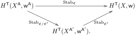### Components/Axes The diagram is structured as a triangle with three nodes and three connecting arrows: **Nodes (Mathematical Expressions):** 1. **Top-Left Node:** \( H^{\top}(X^A, \mathbf{w}^A) \) 2. **Top-Right Node:** \( H^{\top}(X, \mathbf{w}) \) 3. **Bottom Node:** \( H^{\top}(X^{A'}, \mathbf{w}^{A'}) \) **Arrows (Mappings):** 1. **Horizontal Arrow (Top-Left to Top-Right):** Labeled "Stab\(_\epsilon\)". 2. **Diagonal Arrow (Top-Left to Bottom):** Labeled "Stab\(_{\epsilon/\epsilon'}\)". 3. **Diagonal Arrow (Bottom to Top-Right):** Labeled "Stab\(_{\epsilon'}\)". **Spatial Grounding:** * The diagram is centered on a white background. * The three nodes form an inverted triangle: two nodes are aligned horizontally at the top, and the third node is centered below them. * The arrows are straight lines with arrowheads pointing to the target node. The labels are placed approximately at the midpoint of each arrow. ### Detailed Analysis The diagram defines a relationship between three instances of a function or set \( H^{\top} \), each parameterized by a pair \((X, \mathbf{w})\). The superscripts \(A\) and \(A'\) denote different variants or approximations of the primary parameters \((X, \mathbf{w})\). The arrows represent "Stab" (stability) mappings, parameterized by values \(\epsilon\) and \(\epsilon'\). The structure implies that applying the stability mapping Stab\(_\epsilon\) directly from the top-left to the top-right node is equivalent to following the path through the bottom node: first applying Stab\(_{\epsilon/\epsilon'}\) and then Stab\(_{\epsilon'}\). This is the defining property of a commutative diagram. ### Key Observations 1. **Notation:** The use of bold \(\mathbf{w}\) typically denotes a vector, while \(X\) may represent a dataset, design matrix, or another structured input. \(H^{\top}\) could represent a hypothesis class, a loss function, or a set of optimal solutions. 2. **Hierarchy of Approximations:** The diagram suggests a hierarchy where \((X^A, \mathbf{w}^A)\) is an approximation of \((X^{A'}, \mathbf{w}^{A'})\), which in turn is an approximation of the original \((X, \mathbf{w})\). The stability mappings quantify how properties (like solutions or generalization bounds) are preserved under these approximations. 3. **Parameterized Stability:** The stability mappings are not generic but are controlled by specific parameters (\(\epsilon\), \(\epsilon'\), and their ratio \(\epsilon/\epsilon'\)). This indicates a precise, quantifiable relationship between the approximation errors. ### Interpretation This diagram is a formal representation of a **stability-based approximation guarantee**. It visually encodes a theorem stating that if a problem defined by \((X^A, \mathbf{w}^A)\) is stable under the mapping Stab\(_{\epsilon/\epsilon'}\) to an intermediate approximation \((X^{A'}, \mathbf{w}^{A'})\), and that intermediate form is stable under Stab\(_{\epsilon'}\) to the final form \((X, \mathbf{w})\), then the original problem is stable under the composed mapping Stab\(_\epsilon\). **What it means:** In practical terms, this could be used to prove that an efficient algorithm solving an approximate problem (top-left) will produce a solution that is close (within \(\epsilon\)) to the solution of the true, harder problem (top-right). The path through the bottom node provides a way to decompose and analyze the total error \(\epsilon\) into two controllable components, \(\epsilon'\) and \(\epsilon/\epsilon'\). This is a common technique in theoretical computer science and statistical learning theory to establish robustness and generalization bounds for algorithms.

## Diagram Type: Flowchart ### Overview The image depicts a flowchart with arrows indicating the direction of processes or transformations. The chart includes three main components: H^T(X^A, w^A), H^T(X, w), and H^T(X^A', w^A'). Arrows connect these components, suggesting a sequence of operations or relationships between them. ### Components/Axes - **H^T(X^A, w^A)**: This is the starting point of the flowchart. - **H^T(X, w)**: This is the intermediate point, connected by an arrow labeled "Stab_c". - **H^T(X^A', w^A')**: This is the final point, connected by an arrow labeled "Stab_c'". ### Detailed Analysis or ### Content Details - The flowchart shows a transformation from H^T(X^A, w^A) to H^T(X, w) and then to H^T(X^A', w^A'). - The arrow labeled "Stab_c" suggests a stabilization or stabilization process applied to H^T(X^A, w^A) to produce H^T(X, w). - The arrow labeled "Stab_c'" suggests a stabilization or stabilization process applied to H^T(X, w) to produce H^T(X^A', w^A'). ### Key Observations - The flowchart indicates a sequential process with stabilization steps. - The transformation from H^T(X^A, w^A) to H^T(X, w) and then to H^T(X^A', w^A') suggests a transformation or mapping of data or variables. ### Interpretation The flowchart likely represents a process or algorithm where H^T(X^A, w^A) is transformed into H^T(X, w) through a stabilization process, and then further transformed into H^T(X^A', w^A') through another stabilization process. The stabilization processes could be related to data normalization, feature extraction, or other data processing techniques. The exact nature of the transformation and stabilization processes would depend on the specific context and application of the flowchart.

## Mathematical Diagram: Commutative Triangle ### Overview This image is a mathematical diagram, specifically a commutative triangle, illustrating the relationship between three mathematical objects and the maps (morphisms) between them. The objects are denoted by `H^T(...)` and the maps are labeled with `Stab` and subscripts. ### Components and Flow The diagram consists of three nodes and three directed arrows connecting them. * **Nodes (Mathematical Objects):** * **Top-Left Node:** `H^T(X^A, w^A)` * **Top-Right Node:** `H^T(X, w)` * **Bottom Node:** `H^T(X^{A'}, w^{A'})` (Note the period at the end of the expression). * **Arrows (Maps/Morphisms):** * **Horizontal Arrow:** Points from the top-left node `H^T(X^A, w^A)` to the top-right node `H^T(X, w)`. It is labeled `Stab_C`. * **Diagonal Arrow (Down-Right):** Points from the top-left node `H^T(X^A, w^A)` to the bottom node `H^T(X^{A'}, w^{A'})`. It is labeled `Stab_{C/C'}`. * **Diagonal Arrow (Up-Right):** Points from the bottom node `H^T(X^{A'}, w^{A'})` to the top-right node `H^T(X, w)`. It is labeled `Stab_{C'}`. ### Detailed Transcription The textual elements in the diagram are: * `H^T(X^A, w^A)` * `H^T(X, w)` * `H^T(X^{A'}, w^{A'})` * `Stab_C` * `Stab_{C/C'}` * `Stab_{C'}` ### Interpretation The diagram asserts that the composition of the map `Stab_{C/C'}` followed by the map `Stab_{C'}` is equal to the map `Stab_C`. In mathematical notation, this commutativity can be expressed as: `Stab_C = Stab_{C'} ∘ Stab_{C/C'}` This structure is typical in algebraic topology or related fields, where `H^T` likely denotes some form of cohomology (possibly equivariant cohomology, given the `T` superscript), and the `Stab` maps are likely related to stabilization or restriction maps associated with certain conditions or subspaces (denoted by `C`, `C'`, `A`, `A'`). The diagram illustrates a compatibility or factorization property of these maps.

## Diagram: State Transition Model with Stabilization Functions ### Overview The diagram illustrates a state transition model involving three primary states connected by labeled transitions. It uses mathematical notation to represent transformations between states, with stabilization functions governing the transitions. The structure suggests a hierarchical or conditional relationship between the states. ### Components/Axes - **Nodes (States):** 1. $ H^T(X^A, w^A) $: Initial state with parameters $ X^A $ and $ w^A $. 2. $ H^T(X, w) $: Intermediate state with parameters $ X $ and $ w $. 3. $ H^T(X^{A'}, w^{A'}) $: Final state with modified parameters $ X^{A'} $ and $ w^{A'} $. - **Transitions (Arrows):** 1. $ \text{Stab}_\epsilon $: Transition from $ H^T(X^A, w^A) $ to $ H^T(X, w) $. 2. $ \text{Stab}_{\epsilon/\epsilon'} $: Transition from $ H^T(X^A, w^A) $ to $ H^T(X^{A'}, w^{A'}) $. 3. $ \text{Stab}_{\epsilon'} $: Transition from $ H^T(X, w) $ to $ H^T(X^{A'}, w^{A'}) $. ### Detailed Analysis - **Node Labels**: All nodes use the notation $ H^T(\cdot) $, where the arguments vary: - $ X^A, w^A $: Likely represent initial inputs or variables. - $ X, w $: Simplified or transformed inputs. - $ X^{A'}, w^{A'} $: Modified or derived inputs (denoted by primes). - **Transition Labels**: Stabilization functions ($ \text{Stab} $) with subscripts indicating conditions: - $ \epsilon $: A parameter or condition governing the first transition. - $ \epsilon/\epsilon' $: A ratio or comparison between $ \epsilon $ and $ \epsilon' $. - $ \epsilon' $: A modified or secondary condition. ### Key Observations 1. **Flow Direction**: The diagram shows a unidirectional flow from $ H^T(X^A, w^A) $ to $ H^T(X^{A'}, w^{A'}) $, with two possible paths: - Direct path via $ \text{Stab}_{\epsilon/\epsilon'} $. - Indirect path via $ \text{Stab}_\epsilon \rightarrow \text{Stab}_{\epsilon'} $. 2. **Parameter Evolution**: The primes in $ X^{A'} $ and $ w^{A'} $ suggest iterative or conditional updates to the initial parameters. 3. **Stabilization Logic**: The use of $ \text{Stab} $ implies constraints or adjustments to ensure stability during transitions. ### Interpretation This diagram likely models a process where an initial state ($ H^T(X^A, w^A) $) evolves through stabilization mechanisms to reach a refined state ($ H^T(X^{A'}, w^{A'}) $). The two transition paths suggest conditional behavior: - The direct path ($ \text{Stab}_{\epsilon/\epsilon'} $) may represent a shortcut under specific conditions. - The indirect path ($ \text{Stab}_\epsilon \rightarrow \text{Stab}_{\epsilon'} $) could involve intermediate adjustments. The use of stabilization functions ($ \text{Stab} $) implies that the transitions are not arbitrary but governed by constraints (e.g., error correction, optimization). The primes in the final state’s parameters ($ X^{A'}, w^{A'} $) indicate that the process introduces modifications to the original inputs, possibly through feedback or iterative refinement. This structure is common in control systems, optimization algorithms, or machine learning pipelines where states represent model iterations or data transformations. The diagram abstracts the relationships between these stages, emphasizing the role of stabilization in ensuring valid transitions.