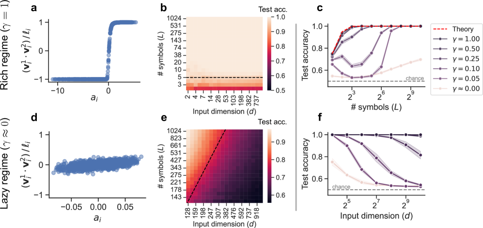
## Performance Analysis of Neural Networks in Different Regimes ### Overview The image presents a comparative analysis of neural network performance under two distinct regimes: a "rich" regime (γ = 1) and a "lazy" regime (γ ≈ 0). The analysis includes scatter plots showing the relationship between input features and a derived quantity, heatmaps illustrating test accuracy as a function of input dimension and number of symbols, and line plots depicting test accuracy versus number of symbols or input dimension for various values of γ. ### Components/Axes **Panel a:** * **Type:** Scatter plot * **X-axis:** `a_i` (values range from approximately -10 to 0) * **Y-axis:** `(v_i^1 * v_i^2) / l_i` (values range from -1 to 1) * **Title:** Rich regime (γ = 1) **Panel b:** * **Type:** Heatmap * **X-axis:** Input dimension (d) with values: 2, 4, 7, 14, 28, 53, 103, 198, 382, 737 * **Y-axis:** # symbols (L) with values: 3, 5, 10, 20, 38, 74, 143, 275, 531, 1024 * **Colorbar:** Test acc. ranging from 0.5 to 1.0 * **Horizontal dashed line:** at # symbols (L) = 5 **Panel c:** * **Type:** Line plot * **X-axis:** # symbols (L) with values: 2^3, 2^6, 2^9 (8, 64, 512) * **Y-axis:** Test accuracy (ranging from 0.6 to 1.0) * **Legend (top-right):** * Dashed red line: Theory * Dark purple line with circles: γ = 1.00 * Purple line with circles: γ = 0.50 * Gray line with circles: γ = 0.25 * Dark gray line with circles: γ = 0.10 * Light gray line with circles: γ = 0.05 * Very light gray line with circles: γ ≈ 0.00 * **Horizontal dashed line:** labeled "chance" at approximately 0.55 **Panel d:** * **Type:** Scatter plot * **X-axis:** `a_i` (values range from approximately -0.05 to 0.05) * **Y-axis:** `(v_i^1 * v_i^2) / l_i` (values range from approximately -0.5 to 0.5) * **Title:** Lazy regime (γ ≈ 0) **Panel e:** * **Type:** Heatmap * **X-axis:** Input dimension (d) with values: 128, 159, 198, 247, 307, 382, 476, 592, 737, 918 * **Y-axis:** # symbols (L) with values: 143, 178, 221, 275, 343, 427, 531, 661, 823, 1024 * **Colorbar:** Test acc. ranging from 0.6 to 0.9 * **Diagonal dashed line:** from bottom-left to top-right **Panel f:** * **Type:** Line plot * **X-axis:** Input dimension (d) with values: 2^5, 2^7, 2^9 (32, 128, 512) * **Y-axis:** Test accuracy (ranging from 0.6 to 1.0) * **Legend:** (Same as Panel c) * Dark purple line with circles: γ = 1.00 * Purple line with circles: γ = 0.50 * Gray line with circles: γ = 0.25 * Dark gray line with circles: γ = 0.10 * Light gray line with circles: γ = 0.05 * Very light gray line with circles: γ ≈ 0.00 * **Horizontal dashed line:** labeled "chance" at approximately 0.55 ### Detailed Analysis **Panel a (Rich Regime):** * The scatter plot shows a clear step function relationship. For `a_i` values less than approximately -2, the `(v_i^1 * v_i^2) / l_i` values are clustered around -1. For `a_i` values greater than approximately 0, the `(v_i^1 * v_i^2) / l_i` values are clustered around 1. There is a sharp transition between these two states. **Panel b (Rich Regime):** * The heatmap shows that high test accuracy (close to 1.0) is achieved for a wide range of input dimensions and number of symbols. Specifically, for # symbols (L) greater than approximately 5, the test accuracy is high regardless of the input dimension. Below # symbols (L) = 5, the test accuracy drops significantly. **Panel c (Rich Regime):** * The line plot shows the test accuracy as a function of the number of symbols for different values of γ. * **Theory (dashed red line):** The theoretical performance reaches a test accuracy of 1.0 at approximately 2^6 symbols. * **γ = 1.00 (dark purple):** The test accuracy increases sharply and reaches 1.0 at approximately 2^6 symbols. * **γ = 0.50 (purple):** The test accuracy increases sharply and reaches 1.0 at approximately 2^6 symbols. * **γ = 0.25 (gray):** The test accuracy increases sharply and reaches approximately 0.95 at 2^9 symbols. * **γ = 0.10 (dark gray):** The test accuracy increases gradually and reaches approximately 0.75 at 2^9 symbols. * **γ = 0.05 (light gray):** The test accuracy remains relatively constant at approximately 0.6. * **γ ≈ 0.00 (very light gray):** The test accuracy remains relatively constant at approximately 0.55, close to the "chance" level. **Panel d (Lazy Regime):** * The scatter plot shows a weak, almost linear relationship. The points are scattered around the origin, with a slight positive correlation between `a_i` and `(v_i^1 * v_i^2) / l_i`. **Panel e (Lazy Regime):** * The heatmap shows that high test accuracy (close to 0.9) is achieved only when both the input dimension and the number of symbols are sufficiently large. The diagonal dashed line separates the region of high accuracy (above and to the right) from the region of lower accuracy (below and to the left). **Panel f (Lazy Regime):** * The line plot shows the test accuracy as a function of the input dimension for different values of γ. * **γ = 1.00 (dark purple):** The test accuracy remains at 1.0. * **γ = 0.50 (purple):** The test accuracy remains at 1.0. * **γ = 0.25 (gray):** The test accuracy remains at 1.0. * **γ = 0.10 (dark gray):** The test accuracy decreases from 1.0 to approximately 0.8 as the input dimension increases. * **γ = 0.05 (light gray):** The test accuracy decreases from approximately 0.9 to approximately 0.7 as the input dimension increases. * **γ ≈ 0.00 (very light gray):** The test accuracy remains relatively constant at approximately 0.6, slightly above the "chance" level. ### Key Observations * In the rich regime (γ = 1), the network exhibits a clear step-function behavior in the relationship between input features and the derived quantity. High test accuracy is achieved with a relatively small number of symbols. * In the lazy regime (γ ≈ 0), the relationship between input features and the derived quantity is weak. High test accuracy requires both a large input dimension and a large number of symbols. * The performance of the network is highly dependent on the value of γ. Higher values of γ lead to better performance, especially in the rich regime. * The "chance" level represents the baseline performance that can be achieved by random guessing. ### Interpretation The data suggests that the rich and lazy regimes represent fundamentally different modes of operation for neural networks. In the rich regime, the network is able to learn a clear and distinct representation of the input data, leading to high accuracy even with a limited number of symbols. In the lazy regime, the network struggles to learn a meaningful representation, requiring a much larger input dimension and number of symbols to achieve comparable accuracy. The value of γ appears to control the transition between these two regimes. As γ increases, the network shifts towards the rich regime, exhibiting better performance and a more distinct representation of the input data. The theoretical performance line in Panel c suggests an upper bound on the achievable accuracy, which is approached by the γ = 1.00 and γ = 0.50 curves. The heatmaps provide a visual representation of the trade-off between input dimension and number of symbols. In the rich regime, a small number of symbols is sufficient to achieve high accuracy, while in the lazy regime, both a large input dimension and a large number of symbols are required. The scatter plots illustrate the underlying behavior of the network in each regime. In the rich regime, the network exhibits a clear step-function behavior, while in the lazy regime, the behavior is more random and less structured.

## Charts/Graphs: Neural Tangent Kernel Regime Performance ### Overview The image presents a series of six sub-plots (a-f) illustrating the relationship between input dimension (d), number of symbols (L), and test accuracy in two different neural network regimes: a "rich" regime (γ = 1) and a "lazy" regime (γ ≈ 0). The plots use scatter plots and heatmaps to visualize these relationships, with a theoretical curve provided for comparison. ### Components/Axes * **Sub-plots a & d:** Scatter plots with `aᵢ` on the x-axis and `(v₁² - v₂²)/lᵢ` on the y-axis. * Sub-plot a is labeled "Rich regime (γ = 1)". * Sub-plot d is labeled "Lazy regime (γ ≈ 0)". * **Sub-plots b & e:** Heatmaps showing "Test acc." (Test Accuracy) as a function of "Input dimension (d)" on the x-axis and "# symbols (L)" on the y-axis. * Sub-plot b corresponds to the "Rich regime". * Sub-plot e corresponds to the "Lazy regime". * **Sub-plots c & f:** Line plots showing "Test accuracy" on the y-axis versus "# symbols (L)" on the x-axis (log scale). * Sub-plot c corresponds to the "Rich regime". * Sub-plot f corresponds to the "Lazy regime". * **Legend (Sub-plot c):** Located in the top-right corner, the legend identifies different curves based on the value of γ (gamma): * Red dashed line: "Theory" * Black line with circles: γ = 0.00 * Dark grey line with squares: γ = 0.05 * Grey line with triangles pointing down: γ = 0.10 * Light grey line with diamonds: γ = 0.25 * Very light grey line with plus signs: γ = 0.50 * Dotted horizontal line: "chance" * **Axis Scales:** The x and y axes use logarithmic scales in some plots (specifically, the number of symbols L in subplots c and f). ### Detailed Analysis or Content Details **Sub-plot a (Rich Regime):** The scatter plot shows a sharp transition in `(v₁² - v₂²)/lᵢ` around `aᵢ = 0`. For `aᵢ < 0`, the value is approximately -1. For `aᵢ > 0`, the value is approximately 1. **Sub-plot b (Rich Regime Heatmap):** The heatmap shows a strong positive correlation between input dimension (d) and test accuracy. As 'd' increases, the test accuracy increases, reaching a maximum value of approximately 1.0. The heatmap also shows that test accuracy increases with the number of symbols (L), but the effect is less pronounced than with the input dimension. * Test accuracy ranges from approximately 0.5 to 1.0. * Input dimension (d) ranges from 2 to 737. * Number of symbols (L) ranges from 2 to 1024. **Sub-plot c (Rich Regime Line Plots):** The line plots show test accuracy as a function of the number of symbols (L). * The "Theory" curve (red dashed) starts at a test accuracy of approximately 0.6 and rapidly increases to 1.0 as L increases. * The γ = 0.00 curve (black circles) closely follows the "Theory" curve. * As γ increases (0.05, 0.10, 0.25, 0.50), the curves shift downward, indicating lower test accuracy for a given number of symbols. * The "chance" line is a horizontal line at approximately 0.6. **Sub-plot d (Lazy Regime):** The scatter plot shows a dense cluster of points around `(v₁² - v₂²)/lᵢ ≈ 0` for all values of `aᵢ` between approximately -0.05 and 0.05. **Sub-plot e (Lazy Regime Heatmap):** The heatmap shows a weaker correlation between input dimension (d) and test accuracy compared to the rich regime. Test accuracy increases slightly with increasing input dimension, but the increase is less dramatic. Test accuracy also increases with the number of symbols (L), but again, the effect is less pronounced. * Test accuracy ranges from approximately 0.6 to 0.9. * Input dimension (d) ranges from 159 to 918. * Number of symbols (L) ranges from 128 to 1024. **Sub-plot f (Lazy Regime Line Plots):** The line plots show test accuracy as a function of the number of symbols (L). * The γ = 0.00 curve (black circles) remains relatively flat, with test accuracy around 0.65-0.7 for all values of L. * As γ increases (0.05, 0.10, 0.25, 0.50), the curves remain close to the "chance" level. * The "Theory" curve is not present in this subplot. ### Key Observations * The "rich" regime (γ = 1) exhibits a strong dependence of test accuracy on both input dimension and the number of symbols. * The "lazy" regime (γ ≈ 0) shows a much weaker dependence on these parameters. * The theoretical curve in the "rich" regime closely matches the experimental results for γ = 0.00. * The "chance" level represents a baseline performance, and the curves for higher values of γ in the "rich" regime fall below this level. * The scatter plots (a and d) visually represent the distribution of values in each regime, highlighting the distinct behavior. ### Interpretation The data suggests a clear distinction in performance between the "rich" and "lazy" regimes of neural network training. In the "rich" regime, the network is able to learn complex representations, leading to high test accuracy as the input dimension and number of symbols increase. This behavior aligns with the theoretical predictions. In contrast, the "lazy" regime exhibits limited learning capacity, resulting in test accuracy that remains close to the "chance" level regardless of the input dimension or number of symbols. This indicates that the network is not effectively utilizing its parameters in this regime. The difference in behavior can be attributed to the value of γ, which controls the learning rate and the degree of parameter updates during training. A higher value of γ (γ = 1) allows for more significant parameter changes, enabling the network to explore a wider range of representations. A lower value of γ (γ ≈ 0) restricts parameter updates, leading to a more conservative learning process and limited representational capacity. The heatmaps and line plots provide a visual representation of these trends, allowing for a clear comparison of performance across different regimes and parameter settings. The outliers and anomalies, such as the downward shift in test accuracy for higher values of γ in the "rich" regime, highlight the importance of carefully tuning the learning rate to achieve optimal performance.

## [Multi-Panel Scientific Figure]: Comparison of Rich (γ=1) vs. Lazy (γ≈0) Learning Regimes ### Overview This image is a composite scientific figure containing six subplots (a-f) arranged in two rows and three columns. The top row (a, b, c) illustrates the "Rich regime (γ = 1)", while the bottom row (d, e, f) illustrates the "Lazy regime (γ ≈ 0)". The figure compares the learning dynamics, generalization performance, and internal representations of a machine learning model (likely a neural network) under these two distinct regimes. The plots include scatter plots, heatmaps, and line graphs. ### Components/Axes **Global Structure:** - **Top Row Title:** "Rich regime (γ = 1)" - **Bottom Row Title:** "Lazy regime (γ ≈ 0)" - **Panel Labels:** a, b, c (top row, left to right); d, e, f (bottom row, left to right). **Panel a (Top-Left):** - **Type:** Scatter plot. - **X-axis Label:** `a_i` - **Y-axis Label:** `(v_i^T · v_i^T) / l_i` - **Y-axis Range:** Approximately -1 to 1. - **X-axis Range:** Approximately -10 to 0. - **Data:** A dense collection of blue points forming a sharp, step-like transition from y ≈ -1 to y ≈ 1 at x ≈ 0. **Panel b (Top-Center):** - **Type:** Heatmap. - **X-axis Label:** `Input dimension (d)` - **X-axis Ticks:** 2, 4, 7, 14, 27, 50, 93, 178, 382, 737. - **Y-axis Label:** `# symbols (L)` - **Y-axis Ticks:** 3, 5, 10, 20, 38, 74, 143, 275, 531, 1024. - **Color Bar Label:** `Test acc.` - **Color Bar Scale:** 0.5 (dark purple/black) to 1.0 (light peach/white). - **Key Feature:** A horizontal dashed black line at approximately L = 5. The heatmap shows high test accuracy (light colors) across most of the space, particularly for larger d and L. **Panel c (Top-Right):** - **Type:** Line graph. - **X-axis Label:** `# symbols (L)` - **X-axis Scale:** Logarithmic, with ticks at 2³, 2⁶, 2⁹. - **Y-axis Label:** `Test accuracy` - **Y-axis Range:** 0.5 to 1.0. - **Legend:** Located in the top-right corner. Contains: - `Theory` (red dashed line) - `γ = 1.00` (dark purple line with circle markers) - `γ = 0.50` (purple line with circle markers) - `γ = 0.25` (lighter purple line with circle markers) - `γ = 0.10` (light purple line with circle markers) - `γ = 0.05` (very light purple line with circle markers) - `γ ≈ 0.00` (lightest purple/pink line with circle markers) - **Horizontal Reference:** A dashed gray line labeled `chance` at y ≈ 0.5. **Panel d (Bottom-Left):** - **Type:** Scatter plot. - **X-axis Label:** `a_i` - **Y-axis Label:** `(v_i^T · v_i^T) / l_i` (same as panel a). - **Y-axis Range:** Approximately -1 to 1. - **X-axis Range:** Approximately -0.05 to 0.05. - **Data:** A dense cloud of blue points centered around y = 0, with no sharp transition. The distribution is roughly symmetric and concentrated. **Panel e (Bottom-Center):** - **Type:** Heatmap. - **X-axis Label:** `Input dimension (d)` - **X-axis Ticks:** 128, 159, 198, 247, 307, 382, 476, 593, 737, 918. - **Y-axis Label:** `# symbols (L)` - **Y-axis Ticks:** 143, 178, 221, 275, 343, 427, 531, 661, 823, 1024. - **Color Bar Label:** `Test acc.` - **Color Bar Scale:** 0.6 (dark purple) to 1.0 (light peach/white). - **Key Feature:** A diagonal dashed black line running from bottom-left to top-right. The heatmap shows a gradient where accuracy is highest (lightest) in the top-left (low d, high L) and lowest (darkest) in the bottom-right (high d, low L). **Panel f (Bottom-Right):** - **Type:** Line graph. - **X-axis Label:** `Input dimension (d)` - **X-axis Scale:** Logarithmic, with ticks at 2⁵, 2⁷, 2⁹. - **Y-axis Label:** `Test accuracy` - **Y-axis Range:** 0.5 to 1.0. - **Legend:** Same as panel c (implied by color and marker consistency). - **Horizontal Reference:** A dashed gray line labeled `chance` at y ≈ 0.5. ### Detailed Analysis **Panel a (Rich Regime Scatter):** The plot shows a clear phase transition. For `a_i < 0`, the normalized inner product `(v_i^T · v_i^T) / l_i` is consistently -1. At `a_i ≈ 0`, there is a sharp, vertical jump to +1, which holds for `a_i > 0`. This indicates a binary, all-or-nothing change in the represented feature. **Panel b (Rich Regime Heatmap):** Test accuracy is generally high (>0.8) across the explored space of input dimension `d` and number of symbols `L`. The horizontal dashed line at L≈5 may indicate a critical threshold for the number of symbols needed for good generalization in this regime. Accuracy appears to saturate near 1.0 for most combinations where L > 5. **Panel c (Rich Regime Lines):** For the rich regime (γ=1.00, dark purple), test accuracy rapidly reaches ~1.0 as the number of symbols `L` increases beyond 2³ (8). As γ decreases (moving to lighter lines), the accuracy for a given `L` decreases, and more symbols are required to achieve high accuracy. The `γ ≈ 0.00` line shows the poorest performance, only slightly above chance for large `L`. The red dashed "Theory" line represents an upper bound or ideal performance. **Panel d (Lazy Regime Scatter):** In contrast to panel a, the data points are scattered in a cloud centered at y=0, with a range of `a_i` values from -0.05 to 0.05. There is no sharp transition, suggesting a more gradual, distributed change in representations. **Panel e (Lazy Regime Heatmap):** The accuracy pattern is fundamentally different from panel b. There is a strong diagonal trend: high accuracy is achieved only when the number of symbols `L` is large relative to the input dimension `d`. The diagonal dashed line likely represents a theoretical boundary (e.g., L ∝ d). Accuracy drops significantly in the region of high `d` and low `L` (bottom-right). **Panel f (Lazy Regime Lines):** For the lazy regime, test accuracy is plotted against input dimension `d`. For all γ values, accuracy *decreases* as `d` increases. The rate of decrease is slower for higher γ values. Even for γ=1.00 (dark purple), accuracy falls from ~1.0 at d=2⁵ to ~0.8 at d=2⁹. For γ≈0.00, accuracy is near chance (0.5) for all `d`. ### Key Observations 1. **Regime Dichotomy:** The "Rich" and "Lazy" regimes exhibit qualitatively different behaviors in representation learning (a vs. d) and generalization scaling (b vs. e, c vs. f). 2. **Phase Transition vs. Gradual Change:** The rich regime shows a sharp, threshold-based transition in its internal metric (panel a), while the lazy regime shows a smooth, centered distribution (panel d). 3. **Scaling Laws:** In the rich regime, generalization improves with more symbols (`L`) and is robust to increasing input dimension (`d`). In the lazy regime, generalization degrades with increasing `d` and requires `L` to scale with `d` to maintain performance. 4. **Role of γ:** The parameter γ acts as a interpolation between regimes. As γ decreases from 1.00 towards 0.00, performance consistently degrades across all metrics, moving from the rich to the lazy regime's characteristics. ### Interpretation This figure demonstrates a fundamental dichotomy in how neural networks can learn, governed by a hyperparameter γ (likely related to initialization scale or learning rate, akin to the "rich" vs. "lazy" or "feature" vs. "kernel" learning regimes in recent literature). - **What the data suggests:** The "Rich regime" (γ=1) enables the model to learn discrete, symbolic representations (evidenced by the sharp transition in panel a) that generalize well and scale efficiently with problem complexity (panels b, c). The model actively shapes its internal features. The "Lazy regime" (γ≈0) results in a model that makes only small adjustments to its initial random features (panel d's cloud). Its generalization is akin to a kernel method, where performance is fundamentally limited by the ratio of symbols to input dimensions (panels e, f), leading to poor scaling with high-dimensional inputs. - **How elements relate:** The scatter plots (a, d) explain the *mechanism* behind the performance curves (c, f) and heatmaps (b, e). The sharp transition in (a) allows for efficient coding and robust generalization, leading to the flat, high-accuracy curves in (c). The diffuse representation in (d) leads to the fragile, dimension-dependent performance in (f). - **Notable anomalies/insights:** The most striking insight is the reversal of the scaling trend with input dimension `d`. In the rich regime, increasing `d` does not harm accuracy (panel b), while in the lazy regime, it is detrimental (panel e, f). This has critical implications for applying such models to high-dimensional real-world data. The diagonal boundary in panel e is a key quantitative finding, suggesting a precise scaling law (L ∝ d) for the lazy regime's capacity.

## Heatmap and Line Graphs: Test Accuracy vs. Input Dimensions and Symbols ### Overview The image contains six subplots (a-f) arranged in a 2x3 grid, analyzing the relationship between input dimensions, number of symbols, and test accuracy under different regimes (rich vs. lazy). Key elements include heatmaps, scatter plots, and line graphs with legends indicating parameter values (γ). --- ### Components/Axes #### Subplot a (Top-Left) - **X-axis**: `a_i` (input dimension) - **Y-axis**: `(v_i^1 · v_i^2)/ℓ_i` (normalized dot product) - **Legend**: - "Rich regime (γ = 1)" (blue line) - "Lazy regime (γ ≈ 0)" (blue dots) - **Spatial Placement**: Legend in top-right corner. #### Subplot b (Top-Center) - **X-axis**: Input dimension (`d`) - **Y-axis**: Number of symbols (`L`) - **Color Scale**: Test accuracy (0.5–1.0, red to yellow) - **Dashed Line**: Horizontal line at `L = 3` (input dimension threshold). - **Legend**: None (colorbar instead). #### Subplot c (Top-Right) - **X-axis**: Number of symbols (`L`) - **Y-axis**: Test accuracy (0.0–1.0) - **Legend**: - Red dashed line: γ = 1.0 (theory) - Purple lines: γ = 0.50, 0.25, 0.10, 0.05 (solid lines) - Light gray dashed line: "chance" (baseline) - **Spatial Placement**: Legend in top-right corner. #### Subplot d (Bottom-Left) - **X-axis**: `a_i` (input dimension) - **Y-axis**: `(v_i^1 · v_i^2)/ℓ_i` (normalized dot product) - **Legend**: - "Lazy regime (γ ≈ 0)" (blue dots) - **Spatial Placement**: Legend in top-right corner. #### Subplot e (Bottom-Center) - **X-axis**: Input dimension (`d`) - **Y-axis**: Number of symbols (`L`) - **Color Scale**: Test accuracy (0.6–0.9, dark red to light red) - **Dashed Line**: Diagonal line at `d = L` (input dimension = symbols). - **Legend**: None (colorbar instead). #### Subplot f (Bottom-Right) - **X-axis**: Input dimension (`d`) - **Y-axis**: Test accuracy (0.0–1.0) - **Legend**: - Purple lines: γ = 1.00, 0.50, 0.25, 0.10, 0.05 (solid lines) - Light gray dashed line: "chance" (baseline) - **Spatial Placement**: Legend in top-right corner. --- ### Detailed Analysis #### Subplot a - **Trend**: A step-like transition from negative to positive values at `a_i ≈ 0`, indicating a regime shift. - **Data Points**: Blue dots cluster near `a_i = 0` for the lazy regime (γ ≈ 0). #### Subplot b - **Trend**: Test accuracy increases with input dimension (`d`) and number of symbols (`L`), but plateaus at `L = 3` (dashed line). - **Key Values**: - At `L = 3`, test accuracy ≈ 0.75 (dashed line). - At `L = 10`, test accuracy ≈ 0.95 (yellow region). #### Subplot c - **Trend**: Test accuracy improves with higher γ values. - γ = 1.0 (red dashed line) achieves near-perfect accuracy (≈ 0.95) for `L ≥ 8`. - Lower γ values (e.g., γ = 0.05) show diminishing returns, with accuracy dropping to ≈ 0.6 for `L = 2`. #### Subplot d - **Trend**: Similar to subplot a but with a broader spread of values for the lazy regime (γ ≈ 0), suggesting less distinct regime separation. #### Subplot e - **Trend**: Test accuracy increases with input dimension (`d`) and number of symbols (`L`), but the diagonal dashed line (`d = L`) marks a critical threshold where accuracy stabilizes. #### Subplot f - **Trend**: Test accuracy improves with higher γ values and input dimension (`d`). - γ = 1.0 (red dashed line) achieves ≈ 0.95 accuracy for `d ≥ 8`. - Lower γ values (e.g., γ = 0.05) show accuracy ≈ 0.6 for `d = 2`. --- ### Key Observations 1. **Regime Separation**: - The rich regime (γ = 1) shows sharp transitions (subplots a, c, f), while the lazy regime (γ ≈ 0) exhibits gradual changes (subplots a, d). 2. **Input Dimension Impact**: - Higher input dimensions (`d`) correlate with improved test accuracy, especially for γ ≥ 0.5 (subplots b, e, f). 3. **Symbol Threshold**: - A critical threshold at `L = 3` (subplot b) and `d = L` (subplot e) marks a plateau in performance. 4. **Chance Baseline**: - The "chance" line (≈ 0.5 accuracy) is consistently below all γ > 0 regimes (subplots c, f). --- ### Interpretation - **γ as a Control Parameter**: Higher γ values (rich regime) enable faster convergence and higher accuracy, particularly for complex input dimensions (`d`) and symbol counts (`L`). - **Input Dimension vs. Symbols**: Test accuracy improves when input dimension (`d`) exceeds the number of symbols (`L`), as seen in the diagonal threshold in subplot e. - **Practical Implications**: - For γ = 1.0, systems achieve near-optimal performance with `d ≥ 8` and `L ≥ 8`. - Lower γ values (e.g., γ = 0.05) require significantly larger input dimensions to match performance, highlighting the trade-off between computational cost and accuracy. - **Anomalies**: - The plateau at `L = 3` (subplot b) suggests a structural limit in the model’s ability to generalize beyond a certain symbol count, regardless of input dimension. This analysis underscores the critical role of γ in balancing model complexity and performance, with practical guidance for optimizing input dimensions and symbol counts.