TECHNICAL ASSET FINGERPRINT
a68994b64e0457288b3db8ea
Click to view fullscreen
Press ESC or click to close
FOUND IN PAPERS
EXPERT: gemini-2.0-flash VERSION 1
RUNTIME: nugit/gemini/gemini-2.0-flash
INTEL_VERIFIED
## Performance Analysis of Neural Networks in Different Regimes
### Overview
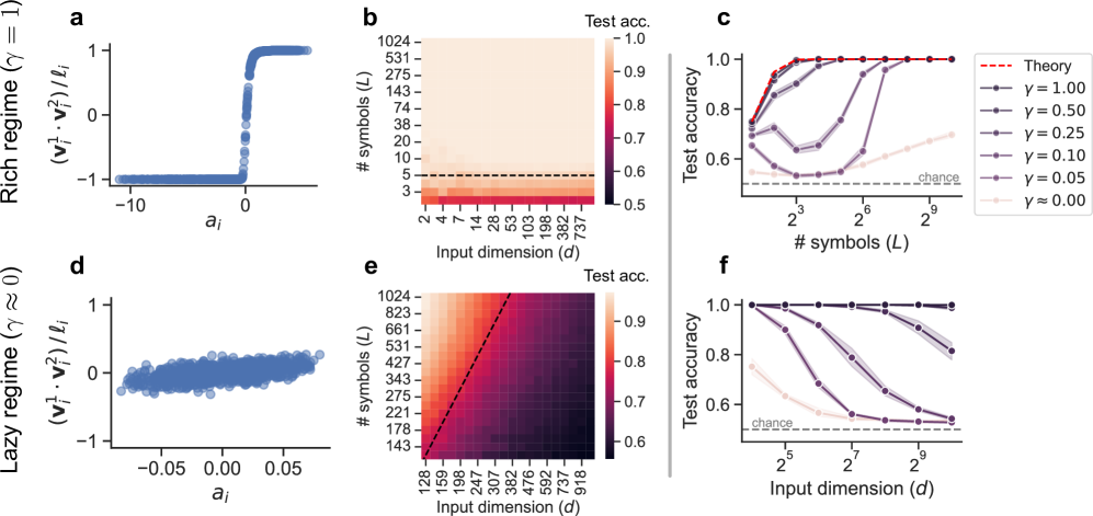
The image presents a comparative analysis of neural network performance under two distinct regimes: a "rich" regime (γ = 1) and a "lazy" regime (γ ≈ 0). The analysis includes scatter plots showing the relationship between input features and a derived quantity, heatmaps illustrating test accuracy as a function of input dimension and number of symbols, and line plots depicting test accuracy versus number of symbols or input dimension for various values of γ.
### Components/Axes
**Panel a:**
* **Type:** Scatter plot
* **X-axis:** `a_i` (values range from approximately -10 to 0)
* **Y-axis:** `(v_i^1 * v_i^2) / l_i` (values range from -1 to 1)
* **Title:** Rich regime (γ = 1)
**Panel b:**
* **Type:** Heatmap
* **X-axis:** Input dimension (d) with values: 2, 4, 7, 14, 28, 53, 103, 198, 382, 737
* **Y-axis:** # symbols (L) with values: 3, 5, 10, 20, 38, 74, 143, 275, 531, 1024
* **Colorbar:** Test acc. ranging from 0.5 to 1.0
* **Horizontal dashed line:** at # symbols (L) = 5
**Panel c:**
* **Type:** Line plot
* **X-axis:** # symbols (L) with values: 2^3, 2^6, 2^9 (8, 64, 512)
* **Y-axis:** Test accuracy (ranging from 0.6 to 1.0)
* **Legend (top-right):**
* Dashed red line: Theory
* Dark purple line with circles: γ = 1.00
* Purple line with circles: γ = 0.50
* Gray line with circles: γ = 0.25
* Dark gray line with circles: γ = 0.10
* Light gray line with circles: γ = 0.05
* Very light gray line with circles: γ ≈ 0.00
* **Horizontal dashed line:** labeled "chance" at approximately 0.55
**Panel d:**
* **Type:** Scatter plot
* **X-axis:** `a_i` (values range from approximately -0.05 to 0.05)
* **Y-axis:** `(v_i^1 * v_i^2) / l_i` (values range from approximately -0.5 to 0.5)
* **Title:** Lazy regime (γ ≈ 0)
**Panel e:**
* **Type:** Heatmap
* **X-axis:** Input dimension (d) with values: 128, 159, 198, 247, 307, 382, 476, 592, 737, 918
* **Y-axis:** # symbols (L) with values: 143, 178, 221, 275, 343, 427, 531, 661, 823, 1024
* **Colorbar:** Test acc. ranging from 0.6 to 0.9
* **Diagonal dashed line:** from bottom-left to top-right
**Panel f:**
* **Type:** Line plot
* **X-axis:** Input dimension (d) with values: 2^5, 2^7, 2^9 (32, 128, 512)
* **Y-axis:** Test accuracy (ranging from 0.6 to 1.0)
* **Legend:** (Same as Panel c)
* Dark purple line with circles: γ = 1.00
* Purple line with circles: γ = 0.50
* Gray line with circles: γ = 0.25
* Dark gray line with circles: γ = 0.10
* Light gray line with circles: γ = 0.05
* Very light gray line with circles: γ ≈ 0.00
* **Horizontal dashed line:** labeled "chance" at approximately 0.55
### Detailed Analysis
**Panel a (Rich Regime):**
* The scatter plot shows a clear step function relationship. For `a_i` values less than approximately -2, the `(v_i^1 * v_i^2) / l_i` values are clustered around -1. For `a_i` values greater than approximately 0, the `(v_i^1 * v_i^2) / l_i` values are clustered around 1. There is a sharp transition between these two states.
**Panel b (Rich Regime):**
* The heatmap shows that high test accuracy (close to 1.0) is achieved for a wide range of input dimensions and number of symbols. Specifically, for # symbols (L) greater than approximately 5, the test accuracy is high regardless of the input dimension. Below # symbols (L) = 5, the test accuracy drops significantly.
**Panel c (Rich Regime):**
* The line plot shows the test accuracy as a function of the number of symbols for different values of γ.
* **Theory (dashed red line):** The theoretical performance reaches a test accuracy of 1.0 at approximately 2^6 symbols.
* **γ = 1.00 (dark purple):** The test accuracy increases sharply and reaches 1.0 at approximately 2^6 symbols.
* **γ = 0.50 (purple):** The test accuracy increases sharply and reaches 1.0 at approximately 2^6 symbols.
* **γ = 0.25 (gray):** The test accuracy increases sharply and reaches approximately 0.95 at 2^9 symbols.
* **γ = 0.10 (dark gray):** The test accuracy increases gradually and reaches approximately 0.75 at 2^9 symbols.
* **γ = 0.05 (light gray):** The test accuracy remains relatively constant at approximately 0.6.
* **γ ≈ 0.00 (very light gray):** The test accuracy remains relatively constant at approximately 0.55, close to the "chance" level.
**Panel d (Lazy Regime):**
* The scatter plot shows a weak, almost linear relationship. The points are scattered around the origin, with a slight positive correlation between `a_i` and `(v_i^1 * v_i^2) / l_i`.
**Panel e (Lazy Regime):**
* The heatmap shows that high test accuracy (close to 0.9) is achieved only when both the input dimension and the number of symbols are sufficiently large. The diagonal dashed line separates the region of high accuracy (above and to the right) from the region of lower accuracy (below and to the left).
**Panel f (Lazy Regime):**
* The line plot shows the test accuracy as a function of the input dimension for different values of γ.
* **γ = 1.00 (dark purple):** The test accuracy remains at 1.0.
* **γ = 0.50 (purple):** The test accuracy remains at 1.0.
* **γ = 0.25 (gray):** The test accuracy remains at 1.0.
* **γ = 0.10 (dark gray):** The test accuracy decreases from 1.0 to approximately 0.8 as the input dimension increases.
* **γ = 0.05 (light gray):** The test accuracy decreases from approximately 0.9 to approximately 0.7 as the input dimension increases.
* **γ ≈ 0.00 (very light gray):** The test accuracy remains relatively constant at approximately 0.6, slightly above the "chance" level.
### Key Observations
* In the rich regime (γ = 1), the network exhibits a clear step-function behavior in the relationship between input features and the derived quantity. High test accuracy is achieved with a relatively small number of symbols.
* In the lazy regime (γ ≈ 0), the relationship between input features and the derived quantity is weak. High test accuracy requires both a large input dimension and a large number of symbols.
* The performance of the network is highly dependent on the value of γ. Higher values of γ lead to better performance, especially in the rich regime.
* The "chance" level represents the baseline performance that can be achieved by random guessing.
### Interpretation
The data suggests that the rich and lazy regimes represent fundamentally different modes of operation for neural networks. In the rich regime, the network is able to learn a clear and distinct representation of the input data, leading to high accuracy even with a limited number of symbols. In the lazy regime, the network struggles to learn a meaningful representation, requiring a much larger input dimension and number of symbols to achieve comparable accuracy.
The value of γ appears to control the transition between these two regimes. As γ increases, the network shifts towards the rich regime, exhibiting better performance and a more distinct representation of the input data. The theoretical performance line in Panel c suggests an upper bound on the achievable accuracy, which is approached by the γ = 1.00 and γ = 0.50 curves.
The heatmaps provide a visual representation of the trade-off between input dimension and number of symbols. In the rich regime, a small number of symbols is sufficient to achieve high accuracy, while in the lazy regime, both a large input dimension and a large number of symbols are required.
The scatter plots illustrate the underlying behavior of the network in each regime. In the rich regime, the network exhibits a clear step-function behavior, while in the lazy regime, the behavior is more random and less structured.
DECODING INTELLIGENCE...